Routing
Introduction
While switching is the mechanism that moves datagrams through a network, routing is the process of determining the routes for datagrams to follow. In the case of circuit switching, cell-switching and virtual circuit switching, the decisions are made when the connection is made; for packet-switching, a decision is made at each router for each packet. In any case, the routers must collect the information and then build their routing tables. If the routing tables are fixed at some point and don't change, they are static routing tables; if the tables change as conditions in the network change, they are dynamic routing tables. If all routing is determined by some central authority that distributed the routing tables to the routers, the routing mechanism is centralized; if each routers determines it own routing tables, the routing mechanism is distributed. We are primarily interested in dynamic, distributed routing methods, but the principles are similar for all types.
Measures of Performance
In determining the best route, you first need to define what you mean by "best". The ideal measure of route desirability would be delivery time, but this turns out to be impractical in many cases. First, clocks on different hosts and routers are not synchronized and may differ by minutes, if not more. Second, determining delivery time by pinging or testing creates significant traffic and isn't reliable. Because situations change rapidly, routers would have to be constantly acquiring new data.
One solution is to use hop count, which is the number of routers that a message will have to go through in order to reach the destination. It is important to note that the message may actually take a different route since each router decides for itself.
Another choice is delay, which measures the expected time that a message will have to wait to be forwarded by a router. This is directly related to the queue length at a particular port or interace. The routers would report an expected cost based on current queue length. Unfortunately, this tends to move packets towards the shortest queue, ignoring the resulting path length.
Transmission time or line latency are other possible choices. They tend to over-emphasize these features. For example, a perfectly good 1 Mbps link looks 100 times worse than a 100 Mbps link, and that tends to skew the routing methods unreasonably. This can be avoided by compressing the dynamic range of these parameters, by, for example, taking the natural log of transmission time.
A hybrid method might include several measures, such as delay, path length and transmission time. For example, the ARPANET revised routing metric is:
Delay = f(QueueTime) + f(TransmissionTime) + f(Latency)
We won't dally any longer on this topic, but it is obviously vital to the robutness and efficiency of the routing method.
Routing Methods
Here are four routing methods that demonstrate some of the choices that might be made:
Source Routing
In this method, the node that sends a packet decides what route the packet should follow, and the routers simply follow the instructions in the packet. The biggest advantage is that the routers only have to do switching on packets. However, the routers are responsible for providing the senders with routing information, so they do have to maintain routing tables. A sender queries the network for a path (and probably creates a connection) and then each packet will contain the path. If the path is broken for some reason, a router will return an error and the sender will have to develop a new route.
Broadcast Routing
The easiest routing method simply has the sender send the packet to all the routers it is connected to and every router does the same. The packet is duplicated and forwarded to all parts of the network very quickly. The advantage is that the packet will quickly find the destination if it exists; the disadvantage is that it takes a lot of network resources. There are some caveats to the broadcast; a router never forwards a message on the port that it arrived on; and the packets usually contain an identifier that allows a router to recognize and discard a packet it has seen before. Broadcast routing is used in very limited situations and where high speed and/or reliability in the face of network failures is very important. Think about a battlefield tactical network system.
Distance Vector Routing
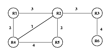
Distance-vector routing provides routes through a process of local exchange. Adjacent routers exchange their routing tables and attempt to build a global view of the network. As an example, consider the following network:
If we consider this network after a period of time, we would see the following routing tables. In this case, we are allowing each router to keep only two routes to any address and only one to any router. Also, it is assumed that the distance from any router to a directly connected network is 1 unit.
|
Routing Table for R1
|
Routing Table for R2
|
| Network |
Distance |
Next Router |
| A |
1 |
Direct |
| B |
1 |
Direct |
| C |
4 |
R2 |
| C |
3 |
R4 |
| D |
7 |
R5 |
| D |
5 |
R2 |
| E |
10 |
R2 |
| E |
5 |
R4 |
|
| Network |
Distance |
Next Router |
| A |
4 |
R4 |
| A |
4 |
R1 |
| B |
4 |
R1 |
| B |
4 |
R1 |
| C |
2 |
R4 |
| C |
5 |
R1 |
| D |
3 |
R5 |
| D |
6 |
R4 |
| E |
8 |
R3 |
|
|
Routing Table for R3
|
Routing Table for R4
|
| Network |
Distance |
Next Router |
| A |
7 |
R2 |
| B |
7 |
R2 |
| C |
5 |
R2 |
| D |
6 |
R2 |
| E |
5 |
R6 |
|
| Network |
Distance |
Next Router |
| A |
3 |
R1 |
| A |
5 |
R2 |
| B |
3 |
R1 |
| B |
5 |
R2 |
| C |
1 |
Direct |
| D |
5 |
R5 |
| D |
4 |
R2 |
| E |
9 |
R2 |
| E |
13 |
R1 |
|
|
Routing Table for R5
|
Routing Table for R6
|
| Network |
Distance |
Next Router |
| A |
6 |
R2 |
| A |
7 |
R4 |
| B |
6 |
R2 |
| B |
7 |
R4 |
| C |
5 |
R4 |
| C |
4 |
R2 |
| D |
1 |
Direct |
| E |
10 |
R2 |
| E |
13 |
R4 |
|
| Network |
Distance |
Next Router |
| A |
11 |
R3 |
| B |
11 |
R3 |
| C |
9 |
R3 |
| D |
10 |
R5 |
| E |
1 |
Direct |
|
Theoretically, a routing algorithm could keep all possible routes, but as you might imagine, the routing tables would get unwieldy quite rapidly. Usually, a router keeps only the shortest few routes, or maybe even the shortes route.
As you can see in the example, the routers build up a table of the routes that they could use. Since this example keeps two routes, if a router or link goes down, a router may have an alternative choice. Or in the interest of balancing the load, it might distribute its traffic over multiple routes.
In order to understand the operation of a distance vector algorithm, consider what happens if another network is added. Assume that network F is added to router R3. R3 will then add R3 at a distance of 1 to its routing table and send that table to its neighbors at R2 and R6. Each of these will add to their routing table at a distance of 4 and 5 respectively. R2 will eventually exchange tables with R1, R2 and R5, so they will add E at distances of 7, 5 and 6 respectively. Finally, R4 exchanges with R1 and R5. R4 now sees two additional routes to E at distances of 9 and 10; it will keep the shorter and put it in the table with the 5 through R2 that it already has. R1 sees another route to E through R4 with the same distance (7) and R5 sees another route to E through R4 with a distance of 9.
Another pertinent example is what happens if the link between R1 and R4 fails. R4 would stop advertising its routes to networks through R1, so R5 would delete these from its routing tables. However, it will eventually add routes that go through R4 and R2. Similarly, R2 would remove the route that it maintains to A and B through R4, and not replace them. Finally, R1 would no longer see R4 as a route to D. Show the new routing tables.
Slow Convergence
One problem with distance-vector routing is that using local information to produce a global perspective can lead to problems. In the example above, if the link between R2 and R3 fails, R2 will set its distance to E to infinity since it goes through R3. But then, it might get a routing table advertisement from R4 indicating that it has a route to R3 with a distance of 9 units. Since routers advertise only destinations and distances with distance-vector routing R2 would not realize that the route depends on its link to R3. R2 may then advertise this new route to R1 and R5. Soon, the entire network would be filled with incorrect routing information. The problem eventually is resolved when R2 passes its table to R4 and R4 changes its distance to E to infinity and the change eventually migrates around the network. The term slow convergence refers to the length of time that might be required for a network of routers to adapt to changing conditions. In this example, the network may have incorrect routing data for some period of time.
To avoid slow convergence, networks can do several things:
- Split Horizon - No node should advertise routes to a router that go through that router. i.e., R4 has a route to E through R2, so it would not advertise that route to R2.
- Poison Reverse - Go ahead and advertise the routes restricted by Split Horizon, but give them a length of infinity.
- Hold Down - When a router loses a link or sees some other major change in the network, it advertises that information, but it doesn't accept any new routes for those destinations for a period of time to insure that the bad news has propagated throughout the network.
Link State Routing
Link-state routing attempts to build routes in a different way. Routers broadcast a list of all the routers to which they have direct connections to every other router in the network. So instead of building a global view based on local information, link-state routing attempts to actually provide the global perspective. Using the example network above, in a stable network, each node would have a table of connectivity and distance information known as an adjacency matrix:
|
R1 |
R2 |
R3 |
R4 |
R5 |
R6 |
A |
B |
C |
D |
E |
| R1 |
0 |
3 |
|
2 |
|
|
1 |
1 |
|
|
|
| R2 |
3 |
0 |
3 |
1 |
2 |
|
|
|
|
|
|
| R3 |
|
3 |
0 |
|
|
4 |
|
|
|
|
|
| R4 |
2 |
1 |
|
0 |
4 |
|
|
|
1 |
|
|
| R5 |
|
2 |
|
4 |
0 |
|
|
|
|
1 |
|
| R6 |
|
|
4 |
|
|
0 |
|
|
|
|
1 |
| A |
1 |
|
|
|
|
|
0 |
|
|
|
|
| B |
1 |
|
|
|
|
|
|
0 |
|
|
|
| C |
|
|
|
1 |
|
|
|
|
0 |
|
|
| D |
|
|
|
|
1 |
|
|
|
|
0 |
|
| E |
|
|
|
|
|
1 |
|
|
|
|
0 |
From this information, each node can create its routing tables by using a method such as Dijkstra's Shortest Path. The nodes get this information by exchanging their connectivity information using reliable flooding, which is another name for broadcast routing. At certain intervals, or when there is a change in its topology, a node broadcasts its connectivity information to all routers in the network. By using this method, the nodes don't rely on local information to build their routes, thereby avoiding problems like slow convergence. The biggest concern with link-state routing is the network capacity required to distribute the tables.