Introduction
A basic sliding window protocol provides the reliability that is necessary for an error-free end-to-end connection, but it doesn't handle two networking problems - flow control and congestion. Flow control is process of managing traffic so that the endpoints themselves are not overwhelmed by the data. This is primarily a problem is one end is much fast than the other and sends data so fast that the other can't process it and clear memory for new messages. It could also happen if one end is simply much busier than the other. Congestion control is the process of managing traffic so that the intervening subnet is not overwhelmed with data for many of the same reasons. Often, routers and/or switches get so busy that they can't process all of the packets arriving. While this sounds more like a problem for the routing and switching algorithm, it is impossible for it to be solved without the cooperation of the endpoints that are supplying all of the packets. This is one place where it is difficult to provide the complete separation between layers that we would like.In order to solve the flow control and congestion control problems, the Transport layer has to be able to identify that a problem exists. Since flow control is strictly a transport layer issue (for transport layer protocols), it can be handled by adding things to the protocol (the header) to allow the endpoints to now conditions on the other end. Of course, the more information you provide, the more complicated the protocol becomes, so you want to limit it as much as possible.
Congestion control is actually a Network layer problem, but it needs some help from the Transport layer and the Transport layer protocol has to have some clues that the problem exists. You could create an interaction between the layers, but that is a complication that makes it difficult to modularize the layers and allow them to work with other protocols, so a better scheme is to use information that is already available. For TCP, that would be packets timing out because they can't get through the subnet in a reasonable time.
Flow Control
The Basic Model
The model used by TCP to control flow is bases on the Effective Window Size or EWS. At any given point in time, the receiving end is providing to the sending end an Advertised Window Size (AWS). This is the amount of data the receiver is willing to accept at any time. The EWS for the sender is:where LBS is Last Byte Sent and LAR is Last ACK Received for the sliding window protocol. The sender never sends more than EWS bytes and the receiver acknowledges every arriving packet with Next Byte Expected and the Advertised Window Size. The AWS decreases if the receiver builds up a backlog of unprocessed data due to a slow application, but it can also change if the receiver finds itself too busy to process data or is running out of memory resources.
For example, the following sequence shows what might happen if you had a very slow receiver in comparison to the sender:
Sender Reciver Event AWS LBS LAR EWS NBE LAS AWS Start 10,000 0 -1 10,000 0 -1 10,000 Send 0-999 10,000 999 -1 9,000 1,000 999 9,000 Send 1000-2999 9,000 2,999 999 7,000 3,000 2,999 7,000 Send 3000-5999 7,000 5,999 2,999 4,000 6,000 5,999 4,000 Send 6000-9999 4,000 9,999 5,999 0 10,000 9,999 0
As you can see, the receiver is acknowledging the receipt of data, but is not able to process it and remove it from the buffer, so the AWS shrinks until it eventually becomes zero and all data transfers halt.
Zero Window Problem
A window size of zero could be a problem. If the sender takes it literally, it might stop sending altogether. If there is no traffic in the other direction, it would never get an updated AWS when it grows. There are a number of ways to solve this problem, but the approach taken in TCP is to make the sender active and the receiver passive. Even if the AWS is zero, the sender continues to send 1-byte packets at regular intervals, which the receiver dutifully acknowledges, thereby getting updated AWS values.Silly Window Syndrome
Another problem TCP might encounter occurs when the receiver is relatively slow at processing data. Its window will go to zero, which it will advertise. Then as it processes data, it will advertise a non-zero but small window, which the sender will promptly fill. So the protocol degrades to sending small segments which is inefficient. In order to avoid the silly window syndrome TCP doesn't advertise windows that are less than 1 MSS in size.Adaptive Retransmission
The next problem to address is the variability in roundtrip response times that you might see in and end-to-end channel. In a subnet where a packet has to travel over many different links and through a corresponding number of routers, the roundtrip or response time can vary greatly. This make is difficult to determine a timeout period to be used for automatic packet resends that won't either be too long or too short. Even if you pick one, it is likely to be obsolete in a matter of seconds due to changing conditions in the network. One strategy that is used is called Adaptive Retransmission. In this scheme, the statistical properties of the network are acquired from the results of previous sends and used to select an appropriate timeout period for the current packet.The basic method uses a smoothing function:
This recursive definition bases the new Estimated Round Trip Time (ERTT) on the previous ERTT and the latest actual value, the Sample Round Trip Time (SRTT). a is a constant in the interval [0,1] that specifies the weight to be placed on each value. A large a places more weight on the previous ERTT and therefore smooths the value more, while a small a is more responsive to changes in the actual round trip times that occur.
For example, if a is 0.6 and we set the initial ERTT to 50 ms, then a sample round trip time of 75 ms would result in an update ERTT of:
If the next roundtrip time was 40 ms, then:
Typical value of a are 0.7 to 1.0.
If this is the roundtrip time you expect, what do you choose for the value of the timeout. Typically, a value of 2 times the ERTT is used. This is conservative, effectively saying that a delay in resending is not as bad as resending an unnecessary duplicate.
Karn/Partridge Algorithm
Adaptive Retransmission works when there aren't any timeouts, but if you get one, now do you measure the roundtrip time; when the acknowledgement arrives, you can't tell if the first packet was received and things were simply slow, or if the duplicate generated the ACK that was received. Since it is impossible to know for sure, the SRTT can't be used with any validity. The Karn/Partridge algorithm suggests that the solution is to assume the worst and simply double the timeout until the ERTT can be recalcuated. For example, if ERTT is 50 ms and the timeout value is 100 ms and a timeout occurs. Double the timeout to 200 ms and continue sending packets. When an acknowledgement for an unduplicated packet arrives in say, 80 ms, that becomes the SRTT and you can calculate a new ERTT. You could multiply by something other than 2 as well.Jacobsen/Karels Algorithm
The previous algorithm works fine, but it fails to take into account the variance in the expected roundtrip time. Another approach is as follows:where typical values are d = 0.5, u = 1 and f = 4. For example, assume that ERTT is 100 and the current deviation is 50, all times in ms:
Most TCP implementations use some form of Jacobsen/Karel's because it provides good reaction to changing conditions in the network, but these are simply choices and are not a defined part of the TCP standard.
Congestion Control
The next problem is congestion control, which is difficult to detect. TCP could certainly take advantage of Source Quench or other ICMP messages, but it prefers to rely on data that is readily available in its own protocol; timeouts and increasing roundtrip times which are good indicators of increasing loads in the network. When these things happen, the TCP senders attempt to slow down their rate of sending and reduce the number of duplicates that they are sending.
The one measure that TCP senders have to control their data rate is the window size. If it shrinks, it forces the sender to more frequently wait for acknowledgements before continuing. The Effective Window Size measures the amount of data that can be allowed, and an additional parameter, the Congestion Window Size is used to reflect the desirability of controlling congestion. In general, the sender will only send up to:
So the CWS can be used to slow down the sender if it is smaller than the EWS. If congestion is a problem (as noted by timeouts and increasing RTT's), decrease CWS, and if not, increase CWS.
Additive Increase Multiplicative Decrease
The congestion avoidance algorithm that is used in implementations of TCP is called Additive Increase Mutliplicative Decrease (AIMD) window management. The idea is that if there is no sign of congestion, you should increase the window size, but not so rapidly as to cause congestion to occur. On the other hand, if congestion appears to be a problem, decrease the window size rapidly to avoid making the problem worse.The algorithm for window management is based on the number of segments that can be sent, which is based on the current segment size. For example, if the window size is 20,000 bytes = minimum {30000, 20000} and the segment size is 500 bytes, then the window size is 20,000/500 = 40 segments.
The algorithm is:
- When an ACK for a full CWS is received, let CWS = CWS + C
- When a timeout occurs, let CWS = CWS * M, where M < 1.0
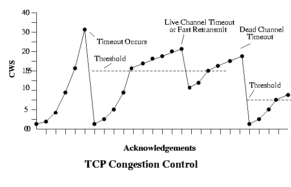
A typical value for C is 1 MSS and 0.5 for M. The following graph shows the changes in the congestion window for this situation.
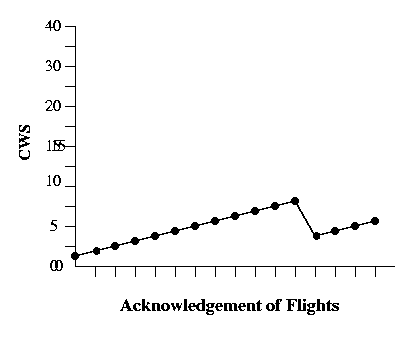
Remember that the increase is based on an acknowledgement for a group of segments representing an entire congestion window size. This would only be an issue for connections moving large amounts of data, but connections moving small amounts of data won't create congestion problems. In a typical instance, the entire group of segments will be sent as a group or flight, and the acknowledgement will return for the entire flight.
Typically, it would be a lot of effort to keep track of the outstanding segments and which are part of a particular congestion window-sized group, so the additive increase is accomplished by adding 1/CWS * MSS, where the CWS is in segments, each time an acknowledgement arrives. CWS acknowledgements will result in an increase of one MSS.
Slow Start
Unfortunately, this is just too slow. Starting at one MSS and building up additively takes too long to get to a reasonable capacity, so another method is used to determine a better starting point. This method is called slow start but it is actually a faster start. It is called slow start because its slower than just starting at the AWS. In slow start, every acknowledgement (not just an acknowledgement for a complete CWS) doubles the congestion window until a timeout occurs. This is called the cold start timeout. A value known as the threshold is then set at one-half of the CWS when the cold start timeout occurs. The CWS is then rolled back to 1 MSS and allowed to grow exponentially again to the threshold, where it then begins to grow additively in the congestion avoidance phase. This process is shown below: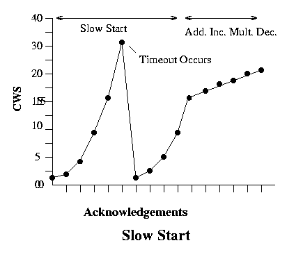
When other timeouts occur there are two possibilities.
- A course-grained or dead-channel timeout occurs when all traffic stops while waiting for a timeout. This means that the entire effective window size has been sent and nothing has been returned, which usually means a signficant delay and possibly major congestion problems.
- A fine-grained or live-channel timeout occurs when there is active traffic but a timeout occurs, usually indicating a more minor problem.
A course-grained timeout means that the entire window has been sent so that the senders window is full, and that data transfer is held waiting for a single acknowledgement at the beginning of the window. If that ACK arrives and the sender responds by sending an entire window, it could have a negative impact on congestion problems in the network. So this type of timeout is handled by performing a complete restart at 1 MSS for the CWS and then entering slow start again. Note that this also resets the threshold value to half the current CWS.
A fine-grained timeout is handled by staying in Additive Increase Multiplicative Decrease collision avoidance mode and dividing the CSW by 2 (typically).
One way to view this process is that given the CWS in segments, when in slow start mode, every acknowledgement adds 1 MSS CWS; when in collision avoidance mode every acknowledgement increases the CWS by 1/CWS times MSS bytes. So for example, given an MSS of 1000 bytes, if the current CWS is 20 and an acknowledgement arrives, if the system is in slow start mode, the new size is 21 segments; if in collision avoidance mode the new size is 20 segments + 1000/20 bytes. Any timeout where there are no incoming acknowledgements or outgoing packets for a period of time causes slow start to be entered, the threshold is set to one-half the CWS and the CWS is set to 1 MSS; any other timeout results in the CWS being halved and slow start being used up to the threshold value and then collision avoidance is started. In the latter case, if the new CWS is above the current threshold, slow start is not used.
In an effort to bring all of these ideas, here is the algorithm for a TCP sender using additive increase-multiplicative-decrease and slow start.
Note that the threshold is never allowed to drop below 2 times MSS. Also, many of these parameters are adjustable depending on the desired properties of your TCP implementation. While the interaction between end-points is carefully defined by TCP, the operation of the endpoints is largely a matter of individual choice. However, the methods described here have been found to work quite well.ACK Received:
if mode == slowstart
CWS = CWS + MSS
if CWS > threshold
mode = aimd
else
CWS = CWS + MSS/CWS
Timeout Event:
threshold = max {CWS/2, 2*MSS}
if no messages in transit /* dead channel */ or in mode == slowstart
CWS = 1
enter mode = slowstart
else // fine-grained timeout
CWS = CWS / 2
if CWS < threshold
mode = slowstart
else
mode == aimd
Fast Retransmit
One condition that might be noticed by the sender is that it gets duplicate ACKS. This might occur because a packet has been lost in transit, so as other packets arrive, the acknowledgements are issued, but they continue to be for the same Next Byte Expected. The Fast Retransmit method tries to avoid an unnecessary timeout by retransmitting the missing packet after three duplicate ACK's, although the three is arbitrary. This is effectively a live-channel timeout since the channel is still busy, and in practice, it has been shown to eliminate about half of the dead-channel timeouts. However, you don't want to ignore the possible congestion implications of the retransmit, so the window should be reduced, but by how much?Fast Recovery
This policy reduces the CWS by half when a fast retransmit occurs.An example of all of this is: