Abiotic Processes: Session I-5

SESSION I-5. MASS TRANSPORT PROCESSES AFFECTING PLUME MIGRATION

The aqueous phase concentration of contaminant resulting from the partitioning process comprises the dissolved contaminant plume which, once established below the water table, is free to move with the ground water. As the plume migrates the concentration of organic contaminants changes with time and space in response to basic mass transport processes including advection, dispersion, sorption (retardation), and possibly biodegradation (additional processes which may affect concentration include volatilization, abiotic degradation, and dilution from recharge occurring along the flow path).

This session contains discussion of each individual mass transport process in both descriptive and mathematical terms. The final result is the one-dimensional transport equation which serves as the basis for the BIOSCREEN model presented in the following session. We begin with a brief review of ground water flow principles followed by discussion of mass transport phenomena.

Ground Water Flow Concepts

It is assumed that students taking this course have had at least some exposure to the basic concepts of flow through porous media. If you need additional back ground in this area a text book on ground water should be referenced. One such popular text is Groundwater by Freeze and Cherry, 1979, as referenced on pg 159 of Wiedemeier.

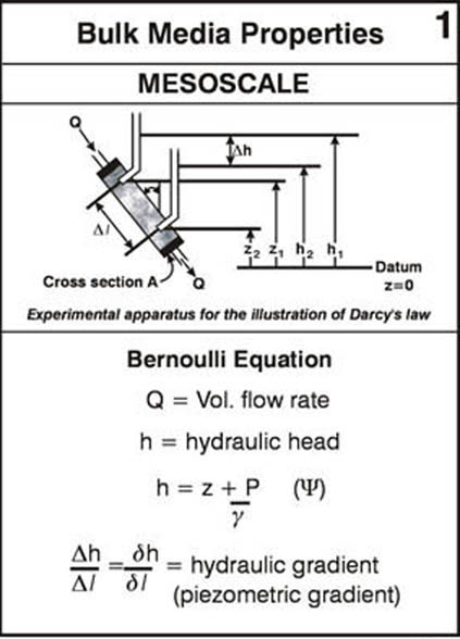
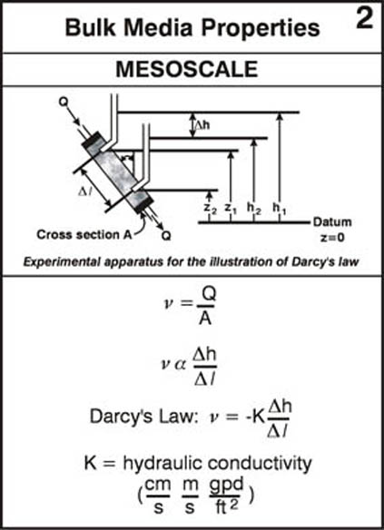
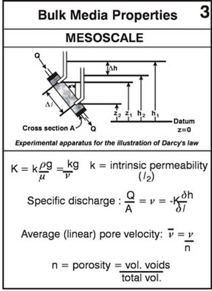
Reading Assignment. In Wiedemeier Chapter 3, please read section 3.1 for background on ground water flow principles. This section discusses Darcy’s law, hydraulic head, hydraulic gradient, hydraulic conductivity, porosity and effective porosity and other basic flow-related principles and concepts.

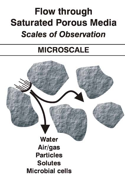
As a supplement to the material in section 3.1 please look over the following annotated figures:

Figure I-5

Figure I-5. If we look at a porous media at a scale small enough to see fluids, particles, solutes, and microbial cells moving through individual pore channels we are observing these phenomena at the “Microscale”. Note that at this scale the focus is on the interactions between fluid, solid, dissolved or suspended constituents in the fluid, and microorganisms attached to the solid surface. Bulk media properties such as permeability, porosity, hydraulic conductivity and dispersivity are not definable at the Microscale.

Figure I-6

Figure I-6. If we consider a large enough sample of porous media, like that shown in the one-dimensional packed-bed flow column above, then it becomes possible to define bulk media properties and equations describing porous media flow.

Figure I-7

Figure I-7. This flowing porous media column represents the experimental apparatus used for the illustration of Darcy’s Law. Note that the Darcian velocity “v” is the total flow rate Q divided by the cross-sectional Area “A”. In other words v is the specific discharge through the one-dimensional porous media column. Note how Hydraulic conductivity K is defined along with typical units.

Figure I-8

Figure I-8. This figure illustrates the relationship between hydraulic conductivity, K, and intrinsic permeability, k. Also note that if the Darcian velocity, v, is divided by the effective porosity n, the result is called the average linear pore velocity.

Figure I-9

Figure I-9. To further explain the concept of average linear pore velocity consider that a conservative tracer (i.e. chloride or non-sportive dye) is added to the column inflow as shown above. Here the tracer is added to the influent as a “step function” or, in other words, the concentration of traced is raised instantaneously from “0” to Co and remains constant thereafter. At the effluent end of the column the tracer breakthrough curve would assume a sigmoidal or “S” shape due to the effects of hydrodynamic dispersion. The time required to for the effluent concentration to reach the centroid of the effluent break through curve is the defined as the “travel time” through the column. Conceptually this represents average travel time, Tt , for tracer to move through the column (some pore channels flow faster, others slower and Tt is the average). The concept which follows here is that average linear pore velocity, as defined in Figure I-8, is equal to the length along the one-dimensional flow path divided by the travel time for the tracer. Note that the actual velocity if water moving through individual porous media flow channels is equal to the average linear pore velocity divided by the tortuosity “T” as shown.

Written Assignment. Questions I-22 through I-25.

Mass Transport through Porous Media

The material on flow through porous media presented in above leads directly into the topic of mass transport, which addresses the processes by which dissolved solutes (“solute” is a generic term which includes all manner dissolved substances including organic contaminants) move through porous media. If you have already had an exposure to the subject of mass transport through porous media the material in this session will serve as a review. If this is your first exposure to the subject please proceed by completing the reading assignment below. The tutorial material presented in this session is intended to provide a more thorough understanding of the basic mass transport concepts of advection, dispersion, sorption, and biodegradation.

Reading Assignment. Pages 130 – 150 address the mass transport processes of advection, molecular diffusion, dispersion, and sorption (retardation). The following written assignment will provide focus. Note that the biodegradation (biotransformation) process is the subject of Chapter 4 in your text and therefore not covered in the current reading assignment. In an effort to provide more complete coverage of the mass transport topic an extensive supplemental reading section is presented below (Mass Transport Processes). This discussion results in the development of the one-dimensional mass transport equation containing process terms for advection, dispersion, sorption and biodegradation. The end result appears as Equation 8.1, page 367 in your text book. Hopefully the development of the complete mass transport equation presented herein will improve basic understanding of how mass transport processes affect spatial and temporal distribution of plume concentration.

Mass Transport Processes

We begin this discussion by writing the complete one-dimensional mass transport equation and defining each term (an example of a “one-dimensional” flow system is given in Figure 3.15, pg 137).

$\frac{\partial C}{\partial t} = \underset{(dispersion)}{D_{L} \frac{\partial^{2} C}{\partial x^{2}}} - \underset{(advection)}{v_{x} \frac{\partial C}{\partial x}} - \underset{(sorption)}{\frac{B_{d}}{n} \frac{\partial C^{*}}{\partial t}} - \underset{(reaction)}{{(\frac{\partial C}{\partial t})}_{r x n}}$

where:

C	=	Concentration of solute in liquid phase	(M/L3 )
t	=	Time
DL	=	Longitudinal Dispersion Coefficient	(L2 /T)
vx	=	Average linear pore velocity	(L/T)
Bd	=	Bulk density of aquifer material	(M/L3 )
n	=	Effective porosity of saturated media
C*	=	Sorbed concentration of solute	(Msolute /Msoil )
rxn	=	Subscript indicating a biological or chemical reaction of solute. In this course this term will be used to represent the time rate of removal of solute (i.e. organic contaminant) from solution due to biodegradation (hence the negative sign in the above equation).

The advantage of writing the transport equation in this form is that each term corresponds to an individual transport process (i.e., advection, dispersion, sorption, and reaction (biodegradation). We will proceed by developing each term in the equation separately. At the conclusion of the session we will refer to the analytical solutions to the one–dimensional transport equation which are presented in Wiedemeier Chapter 4. These analytical solutions serve as the basis for the BIOSCREEN spread sheet model presented in the following session.

The mass transport equation can be explained by visualizing a stationary point located in a one-dimensional porous media flow field. Note that the term “one-dimensional” means that the flow velocity vector, vx , has only one component. Now assume that the groundwater passing by the stationary point has a variable concentration “C” of dissolved solute, for example an organic contaminant such as TCE. The transport equation indicates that the partial derivative of C with respect to time will be governed by the combined effects of individual mass transport processes including dispersion, advection, sorption and reaction (i.e. biodegradation). Specifically the time rate of change of “C” will increase due to dispersion and decrease due to the effects of advection, sorption and biodegradation. The following section will analyze each of these transport processes separately with the intention of providing an in-depth understanding of each transport process.

Hydrodynamic Dispersion

The first process we will consider is hydrodynamic dispersion. Conceptually hydrodynamic dispersion is the sum of the effects of molecular diffusion plus mechanical dispersion (pg 130-134).

Molecular Diffusion. Molecular diffusion is the process by which dissolved molecular species move from regions of high concentration to regions of low concentration. The diffusion of a dissolved solute through water is described by Fick’s first law. According to Fick’s first law the steady state mass flux through a one-dimensional flow system is given by Equation 3.8, pg 131:

$F = - D_{d} (\frac{d C}{d x})$

Where:

F	=	Mass flux of solute per unit area per unit time	(ML/T)
Dd	=	Diffusion coefficient	(L2 /T)
C	=	Solute concentration	(M/L3 )
$\frac{d C}{d x}$	=	Spatial concentration gradient along the axis of flow path	(M/L3 /L)

The negative sign indicates that the movement is from greater to lesser concentrations. Values for Dd are well known . For major cations and anions in water Dd ranges from 1 x 10-9 to 2 x 10-9 m2 /s.

In porous media diffusion cannot proceed as fast as it does in water because the ions must follow longer pathways as they travel around media particles. To take this into account an effective (porous media) diffusion coefficient must be used. This is termed D*, which can be determined from the relation:

$D^{*} = ω D_{d}$

Where ω is an empirical coefficient that is determined by laboratory experiment. Observed values for ω range between 0.01 to 0.5.

For molecular diffusion in systems where the concentrations at a point is changing with time Fick’s second law applies:

$\frac{\partial C}{\partial t} = D_{d} \frac{\partial^{2} C}{\partial x^{2}}$

Fick’s second law equation is used to model hydrodynamic dispersion in porous media. This is accomplished by defining the coefficient “D” to include the effects of molecular diffusion plus mechanical dispersion as shown below.

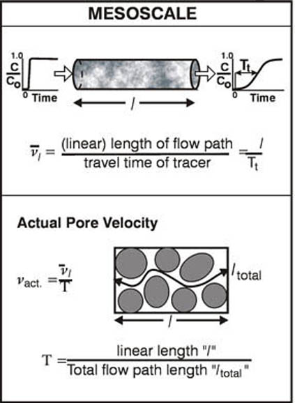
Mechanical Dispersion. Mechanical dispersion results when dissolved solute moves through porous media at velocity vx . Three basic causes of mechanical dispersion are illustrated in Figure 3.11, pg 132. 1) As fluid moves through pores it will move faster through the center of the pore than at the edges (hydrodynamic boundary layer effect). 2) Some of the fluid particle will travel along longer paths in the porous media than other particles to go the same linear distance (tortuosity effects). 3) Some pores are larger than others which allows the fluid flowing through these pores to move faster. It is assumed that mechanical dispersion can be described by Fick’s second law of diffusion, provided that the coefficient “D” is defined to include the effects of fluid velocity. This leads to the definition of the Hydrodynamic Dispersion Coefficient, DL , which is:

$D_{L} = α_{L} v_{x} + D^{*}$

Where:

DL	=	Hydrodynamic Dispersion Coefficient	(L2 /T)
αL	=	Hydrodynamic Dispersivity	(L)
vx	=	Average pore velocity	(L/T)
D*	=	Porous Media Molecular Diffusion Coefficient	(L2 /T)

The term αLvx is referred to as the Mechanical Dispersion Coefficient and indicates that the amount of mechanical dispersion is a function of the average pore velocity. The dynamic dispersivity (or simply “dispersivity”), αL is a property of the porous medium and is scale dependent. The following empirical equation is used to estimate αL :

$α_{L} = 0.1 x$

Where “x” is the linear distance, measured along the axis of the groundwater flow path, between two points between which dispersion is being calculated or measured. For example, if dye tracer is injected into a laboratory column and the tracer breakthrough curve measured at the downstream end of the column, the distance “x” used to calculate dispersion would be the length of the column. Similarly in the field, if the concentration of dissolved contaminant is being calculated at a point 100 feet down gradient from the source area for the contamination, then the relevant value of “x” would be 100 feet. Please note than an alternative equation for estimating αL is given in equation 3.12 pg 134. Equation 3.12 is probably the better choice for most field-scale applications.

Using the above definition for the hydrodynamic dispersion coefficient, DL , Fick’s second law is rewritten to model hydrodynamic dispersion through porous media:

$\frac{\partial C}{\partial t} = D_{L} \frac{\partial^{2} C}{\partial x^{2}} (Hydrodynamic Dispersion Equation)$

It is also important to understand that DL describes hydrodynamic dispersion in the direction parallel to the principal direction of groundwater flow. As a dissolved solute plume moves down gradient it also disperses or “spreads out” in the transverse and vertical directions. Thus the hydrodynamic dispersion concept applies in these orthogonal directions also and leads to the corresponding definitions of hydrodynamic dispersion coefficient and dispersivity shown below:

DT	=	Hydrodynamic dispersion coefficient perpendicular to the principal direction of groundwater flow (transverse).
DZ	=	Hydrodynamic dispersion coefficient in the vertical direction relative to the principal groundwater flow direction.
αT	=	Transverse dispersivity
αZ	=	Vertical dispersivity

Advection

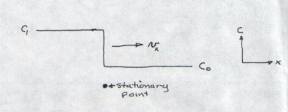
The next term in the in the 1-dimensional mass transport equation is advection. This term describes the time rate of change of concentration occurring at a stationary point due to passing of a dissolved solute “wave” moving at velocity vx . To visualize the advection process refer to the Figure I-10 which shows a “step function” change in solute concentration from C0 up to C1 . Note that the step change in concentration is moving like a “wave” with velocity vx in the x direction.

Figure I-10

Figure I-10. Step Function change in solute concentration moving with velocity vx .

At the instant this concentration wave passes by the stationary point shown, the time rate of change of concentration at that point due to advection is given by:

$\frac{\partial C}{\partial t} = - v_{x} \frac{\partial C}{\partial x} (Advection Equation)$

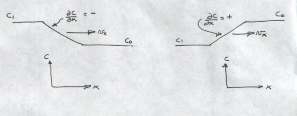
In differential terms $v_{x} = \frac{\partial x}{\partial t}$ , therefore dimensionally $- \frac{\partial x}{\partial t} \frac{\partial C}{\partial x} = \frac{\partial C}{\partial t}$ . In other words when the concentration change, moving at velocity vx reaches the stationary point, the time rate of concentration observed at that point will be equal to the product of the velocity times the spatial concentration gradient in the x direction. The negative sign in the advection appears because the spatial concentration gradient, $\frac{\partial C}{\partial x}$ can either be positive or negative. Examples of concentration profiles with positive and negative spatial gradients are shown in Figure I-11.

Figure I-11

Figure I-11. Concentration profiles with positive and negative spatial gradients.

Combining Advection and Dispersion. Combining the advection and dispersion processes results in the following equation, which is the same as Equation 3.14, pg136.

$\frac{\partial C}{\partial t} = D_{L} \frac{\partial^{2} C}{\partial x^{2}} - v_{x} \frac{\partial C}{\partial x} (Advection - Dispersion Equation)$

An analytical solution to the advection/dispersion equation is presented in Example 3.3, pg 136.

Written Assignment: Questions I-26, I-27.

Sorption

Reading Assignment. Please read section 3.4, pg 138 – 150. The following discussion will provide more in-depth coverage of the sorption topic.

Linear Sorption Isotherm. Sorption is the next mass transport process considered here. The development of the sorption term in the 1-dimensional mass transport equation is based on the concept of the linear sorption isotherm, which is discussed on pg 142 and again in the Equilibrium Partitioning session of this course. The linear sorption isotherm is described by the equation:

$C^{*} = K_{d} C (Linear Sorption Isotherm Equation)$

Where:

C*	=	Mass of solute per dry unit mass of soil	(common units: mg/Kg)
C	=	Concentration of solute in solution (in the pore water) in equilibrium with the mass of solute sorbed on the soil	(common units: mg/L)
Kd	=	Distribution coefficient	(common units: (L/kg)

The linear sorption isotherm equation assumes that, at equilibrium, the solute concentration, C, in the pore water is directly proportional to the sorbed concentration, C* , and Kd is the proportionality constant. Note that the linear sorption isotherm is but one of several possible equations which are commonly used to model the sorption behavior of contaminants in aquifers.

Other relationships including the Freundlich and Langmuir sorption isotherms, are discussed on pages 140 - 141. Note that these isotherms are non-linear in nature (and very likely more representative of the complexities encountered with soil – organic interactions). The fact that the linear sorption isotherm is used in the development of the mass transport equation represents a major assumption. Any calculations made using equations involving the retardation factor “R” (this include the BIOSCREEN model) are based on the assumption of a “linear” sorption isotherm.

It is further assumed that sorption of organic solutes (contaminants) occurs only on the fraction of soil containing organic carbon (foc ). Therefore the distribution coefficient is modeled as:

$K_{d} = f_{o c} K_{o c}$

Where:

foc	=	The fraction (by weight) of aquifer soil composed of organic carbon (decimal fraction)
Koc	=	Soil sorption (distribution) coefficient normalized for total organic carbon content. See pg 145-146.	(common units: L/kg)

Contribution to $\frac{\partial C}{\partial t}$ from Sorption. As dissolved hydrophobic organic molecules move through soil pores they are attracted to binding sites such as the organic carbon material in the soil. Therefore organic molecules initially leave the aqueous phase and sorb to the solid phase thereby decreasing the initial aqueous phase concentration, C, and increasing the sorbed concentration, C* . This process continues until chemical equilibrium is reached. From the basic dynamics of the sorption process it can be assumed that the time rate of change of dissolved concentration at a stationary point is balanced by the time rate of change sorbed concentration at that point. Therefore, if we assume instantaneous equilibrium at the point we can write the following: $\frac{\partial C}{\partial t} = f (\frac{\partial C^{*}}{\partial t})$

If we examine the fundamental dimensions of each term in the above equation we have:

$\frac{\partial C}{\partial t} = \frac{M_{s o l u t e}}{V_{l i q u i d} T}$

$\frac{\partial C^{*}}{\partial t} = \frac{M_{s o l u t e}}{M_{s o i l} T}$

In order for the dimensions for $\frac{\partial C}{\partial t}$ and $\frac{\partial C^{*}}{\partial t}$ to balance we must multiply the units of $\frac{\partial C^{*}}{\partial t}$ by $\frac{M_{s o i l}}{V_{l i q u i d}}$ as follows:

$(\frac{M_{s o l u t e}}{M_{s o i l} T}) (\frac{M_{s o i l}}{V_{l i q u i d}}) = \frac{M_{s o l u t e}}{V_{l i q u i d} T}$ , which are the dimensions for $\frac{\partial C}{\partial t}$ . Now replace $V_{l i q u i d}$ with the term $V_{s o i l} n$ , where n is porosity. Here we assume that for saturated conditions, the volume of water in the pore space, $V_{l i q u i d}$ , is equal to the volume of soil, $V_{s o i l}$ , multiplied by the porosity, n. This results in the following rearrangement:

$(\frac{M_{s o l u t e}}{M_{s o i l} T}) (\frac{M_{s o i l}}{V_{s o i l} n})$ , and since $(\frac{M_{s o i l}}{V_{s o i l}})$ is the soil bulk density, $B_{d}$ , the resulting dimensional analysis becomes:

$(\frac{M_{s o l u t e}}{M_{s o i l} T}) (\frac{B_{d}}{n}) = \frac{M_{s o l u t e}}{V_{l i q u i d} T}$ which shows that:

$\frac{\partial C}{\partial t} = - \frac{B_{d}}{n} \frac{\partial C^{*}}{\partial t} (Sorption Equation in terms of C^{*})$

The minus sign indicates that if $\frac{\partial C^{*}}{\partial t}$ is increasing then $\frac{\partial C}{\partial t}$ must be decreasing.
Since $C^{*} = K_{d} C$ , the sorption equation for 1-dimensional mass transport can also be written:

$\frac{\partial C}{\partial t} = - K_{d} \frac{B_{d}}{n} \frac{\partial C}{\partial t} (Sorption Equation in terms of C)$

Combining Advection, Dispersion and Sorption. The 1-dimensional mass transport equation accounting for advection, dispersion and sorption can be written either as:

$\frac{\partial C}{\partial t} = D_{L} \frac{\partial^{2} C}{\partial x^{2}} - v_{x} \frac{\partial C}{\partial x} - \frac{B_{d}}{n} \frac{\partial C^{*}}{\partial t} (Advection-Dispersion-Sorption Eq . in terms of C^{*})$

or as:

$\frac{\partial C}{\partial t} = D_{L} \frac{\partial^{2} C}{\partial x^{2}} - v_{x} \frac{\partial C}{\partial x} - K_{d} \frac{B_{d}}{n} \frac{\partial C}{\partial t} (Advection-Dispersion-Sorption Eq . in terms of C^{})$

Derivation of Retardation Factor, R. The retardation factor can be derived as follows:

$\frac{\partial C}{\partial t} = D_{L} \frac{\partial^{2} C}{\partial x^{2}} - v_{x} \frac{\partial C}{\partial x} - K_{d} \frac{B_{d}}{n} \frac{\partial C}{\partial t}$

can be rearranged as:

$\frac{\partial C}{\partial t} (1 + K_{d} \frac{B_{d}}{n}) = D_{L} \frac{\partial^{2} C}{\partial x^{2}} - v_{x} \frac{\partial C}{\partial x}$

and if we define retardation factor as

$R = (1 + K_{d} \frac{B_{d}}{n})$

and the equation above becomes:

$\frac{\partial C}{\partial t} R = D_{L} \frac{\partial^{2} C}{\partial x^{2}} - v_{x} \frac{\partial C}{\partial x}$

Now if we neglect the effects of dispersion, this equation becomes:

$R = - v_{x} \frac{\partial C}{\partial x} \frac{\partial t}{\partial C} = - v_{x} \frac{\partial t}{\partial x}$

in which the term $\frac{\partial t}{\partial x}$ is conceptually the reciprocal of vc , which is the average velocity of the solute front. This means retardation factor is in fact the ratio of fluid velocity, vx , to the velocity of the solute front vc :

$R = \frac{v_{x}}{v_{c}} = (1 + K_{d} \frac{B_{d}}{n}) (Retardation Equation)$

Note that the negative sign disappears because the spatial gradient $\frac{\partial C}{\partial x}$ is always negative in a system where the solute velocity is less than the fluid velocity. The main concept here is that, if a hydrophobic organic compound is moving with ground water flow, the solute will move in the same direction as the water. However, because solute molecules are being transferred for the aqueous phase to the solid phase due to sorption, the velocity of the solute front is reduced relative to the fluid velocity. Thus if sorption is negligible (i.e., Kd = 0), then R = 1 and this means that the solute (contaminant) is moving at the same average linear velocity as the pore water. If, for example, R were equal to 2, then this would mean that the pore water is moving with twice the velocity of the solute front.

Written Assignment: Question I-28.

Mass Transport Equation in Terms of R. It should be noted that the one-dimensional mass transport equation, in terms of advection, dispersion, and sorption, can also be written in terms of retardation factor, R as:

$\frac{\partial C}{\partial t} R = D_{L} \frac{\partial^{2} C}{\partial x^{2}} - v_{x} \frac{\partial C}{\partial x}$

or also as:

$\frac{\partial C}{\partial t} = \frac{D_{L}}{R} \frac{\partial^{2} C}{\partial x^{2}} - \frac{v_{x}}{R} \frac{\partial C}{\partial x}$

This is the same as Equation 3.28, 150.

Biodegradation. The biodegradation (or biotransformation) term in the one-dimensional mass transport equation represents the rate at which solute mass is removed from solution due to biodegradation. This is expressed as:

$\frac{\partial C}{\partial t} = {(\frac{\partial C}{\partial t})}_{r x n}$

When the reaction is due to biodegradation or biotransformation of the organic solute the “zero order” and “first order” models are commonly used:

${(\frac{\partial C}{\partial t})}_{r x n} = B (Zero Order Biodegradation Rate Equation)$

Where B is a constant with units M/V/T (e.g. mg/L/day). B is considered “zero order” with respect to solute concentration. The First Order model is:

${(\frac{\partial C}{\partial t})}_{r x n} = λ C (First Order Biodegradation Rate Equation)$

Where:

λ	=	First order decay rate constant (T-1 )	Common units are 1/days, or 1/years
C	=	Solute (contaminant) concentration (M/V/T)	Common units: mg/L

The Monod kinetic model discussed on pg 183-186 Wiedemeier is also an alternative modeling the biodegradation term. However this equation requires that the specific growth rate characteristics of the microbial consortia be defined along with the total microbial population per unit volume of aquifer material. As such the Monod kinetic model is more useful for analyzing biodegradation occurring under very controlled (laboratory) conditions and thus has limited application under field conditions.

Summary of Mass Transport Equations

The foregoing derivations of individual mass transport terms can be combined resulting in the mass transport equation which describes the movement of a sorptive, reactive (i.e. biodegradable), dissolved solute in a 1-dimensional velocity through porous media. This equation is written:

$\frac{\partial C}{\partial t} = \underset{(dispersion)}{D_{L} \frac{\partial^{2} C}{\partial x^{2}}} - \underset{(advection)}{v_{x} \frac{\partial C}{\partial x}} - \underset{(sorption)}{K_{d} \frac{B_{d}}{n} \frac{\partial C}{\partial t}} - \underset{(biodegradation)}{λ C} (Mass Transport Eq .)$

where:

C	=	Concentration of solute in liquid phase	(M/L3 )
x	=	Distance along the principal axis of flow	(L)
T	=	Time	(T)
DL	=	Longitudinal Dispersion Coefficient	(L2 /T)
vx	=	Average linear pore velocity	(L/T)
Bd	=	Bulk density of aquifer material	(M/L3 )
n	=	Effective porosity of saturated media	(V/V)
λ	=	First order decay rate constant. Common units are 1/days, or 1/years	(T-1 )
Kd	=	Distribution coefficient (common units: (L/kg)	(V/M)

This formulation describes how the time rate of change of solute concentration at a stationary point changes due the combined effects of the individual mass transport processes of advection, dispersion, sorption, and biodegradation. Note that the zero order model for biodegradation rate could also be substituted in place of the first order term.

The 1-dimensional mass transport equation can also be rearranged and written in terms of the retardation factor, R, as:

$\frac{\partial C}{\partial t} = \frac{D_{L}}{R} \frac{\partial^{2} C}{\partial x^{2}} - \frac{v_{x}}{R} \frac{\partial C}{\partial x} - λ C (Equation 8 .1, Wiedemeyer)$

This version of the transport equation corresponds to Equation 8.1 on pg 366. Analytical solutions for solute transport are presented in Wiedemeier (pg 367-387). Variations of equation 8.1, written for 1, 2 and 3 dimensions, form the basis for these analytical solutions. The BIOSCREEN model presented in the following session is based on an analytical solution to the three-dimensional version of Equation 8.1.

Natural Attenuation. The foregoing material in session I-5 provides excellent background to introduce the concept of “Natural Attenuation” which along with pump-and-treat, soil vapor extraction, soil excavation, and phytoremediation, represent most of the commonly-used remediation strategies, The major concept behind natural attenuation is that the naturally occurring mass transport process of advection, dispersion, sorption and biotransformation act to reduce the concentration of dissolved contaminant concentration as the plume migrates down-gradient. The appropriateness of natural attenuation as an acceptable remediation alternative depends heavily on individual site conditions. In the case where threat to human health is not perceived to be a factor, natural attenuation may be considered as a remediation option. If so, then a comprehensive program of field monitoring must be instituted in order to track the progress of the dissolved plume with time. Ideally such a monitoring program should ultimately demonstrate that the plume is becoming stable in size and hopefully shrinking. Note that the term Monitored Natural Attenuation (MNA)” is frequently used to in discussing this remediation strategy.

Reading Assignment. Read Chapter 1, pages 1through 26. This will provide an good overview of natural attenuation.

Next Session