From Machine Code to High-Level Languages

A program today is written in a high-level language and reaches the processor through a stack of abstractions: libraries, a compiler or an interpreter, an instruction set, and a microarchitecture underneath that. Every one of those layers was put there by somebody, for a reason, and often over somebody else’s objection.

These abstractions have not always existed. The earliest stored-program machines were programmed by putting bits into the store directly. On the Manchester Baby, in June 1948, that meant stepping through the store word by word and setting each bit to 0 or 1 on a device of 32 buttons and switches: the first program to run there was seventeen instructions long and written one bit at a time.

Those bits formed a language. They were broken up into words, each corresponding to a single instruction, which the machine read and executed one by one. Every word had a fixed shape, each part of that shape meant something, and the machine combined those meanings by fixed rules — a vocabulary and a grammar.

What makes this language of bits low-level is that its vocabulary is the machine’s own. The only thing a word can say is that the hardware should carry out one of its operations, and a program is a sequence of such words — so there is no shortage of computations you can express in it. What has nowhere to go is everything you understand about the program besides the operations themselves. That these twelve words are a routine for computing a square root; that location 90 holds a running total; that this jump is the one closing a loop; that the words further down are data rather than instructions — none of it is recorded in the store, because the notation has nothing to record it with. It lived in pencil annotations on the paper beside the machine, and in the programmer’s memory. The rest of this chapter explores how languages evolved to move more of that intent into the program itself.

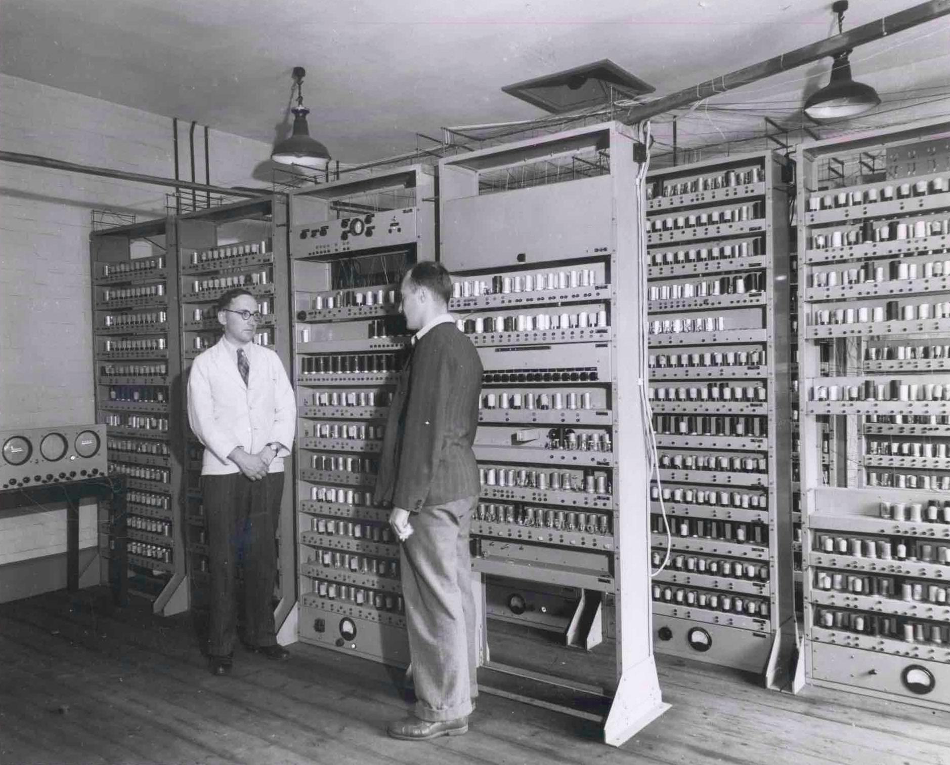
Consider one of the earliest machines to make such a move. The EDSAC ran at Cambridge from May 1949. The EDSAC took about 1.5 milliseconds to execute an order (approximately 650 orders a second). On the first morning the EDSAC was running, it took two minutes and thirty-five seconds to compute and print a table of the first 100 perfect squares (0 to 9801).

The EDSAC’s store held words consisting of 17 bits. An instruction — an order, in the vocabulary of the time — occupied exactly one such word, divided into four fields:

      5 bits      1        10 bits       1
   ┌───────────┬───────┬──────────────┬────────┐
   │  function │ spare │   address    │ length │
   └───────────┴───────┴──────────────┴────────┘

Here is an example of one such order as a sequence of 17 bits:

   1 1 1 0 0    0    0 0 0 1 0 1 1 0 1 0    0
   ─────────    ─    ───────────────────    ─
    function  spare         address       length

Function 11100, address 0001011010 — 90 in decimal — and a length bit of 0. The order instructs the machine to add the number held in location 90 to the accumulator. While this is how orders are represented and understood by the machine, it is not how one wrote programs for EDSAC. A programmer would write a sequence of characters representing the orders to be executed onto a paper tape that EDSAC read into its store and then ran. Below is an example program that represents a small routine that divides by repeated subtraction, leaving the remainder in location 92. The left-hand column depicts where the order is stored, the middle column is the sequence of characters that encode the order, and the right column describes what the order does.

 store     order      description
   56      A 90 F     add the number in location 90 into the accumulator
   57      S 91 F     subtract the number in location 91 from the accumulator
   58      E 57 F     if the accumulator is positive, continue at location 57
   59      T 92 F     store the accumulator into location 92 and clear it

While the above structured representation is helpful to understanding the procedure, the actual program written to the paper tape didn’t contain the store location of instructions, the description or any white space. The tape would simply read A90FS91FE57FT92F and then relied on being loaded into the store from location 56 onward.

The description in that third column, and everything else a reader would need, sat outside the tape entirely. What a routine was for lived on its manuscript — a separate sheet, written out by hand, setting out the same orders with commentary beside them. Even the program’s name was kept outside the program: the practice was to write it on the tape in pencil.

The gap between the bits in the store and the characters on the tape is smaller than it appears. A paper tape records characters as five-bit teleprinter codes, and an order’s function field is five bits wide — so the order code was numbered to make the two coincide. 11100 is at once the function code for add and the teleprinter code for the letter A; 01100 is both subtract and the letter S. The letter punched on the tape was the function field, already in binary, with nothing to convert. As Martin Campbell-Kelly writes in his Tutorial Guide to the EDSAC Simulator, this “simplified the translation of the symbolic program considerably.” It is an early instance of hardware being shaped around the convenience of programming: the order code was numbered to suit the notation a person would write on the tape.

The addresses got no such help, and that is where the difficulty lived. 90, 91, 92, and 57 are absolute store locations, fixed at the moment the routine was written. Suppose you now need one more order between the ones at 57 and 58. Everything below the insertion shifts down a word: the two remaining orders move to 59 and 60, and the three numbers this routine works on, held after the program, move to 91, 92, and 93. So A 90 F, S 91 F, and T 92 F must each have their address increased by one, by hand, in the listing. The jump E 57 F points backward, to a location before the insertion, and must be left exactly as it is.

Note which orders those were. The branch is the one you would think to check, and it is the one that turns out to be fine; the arithmetic orders are what broke, because the data moved even though nothing about the arithmetic changed. That is the whole difficulty in one observation, and it is the documented reason the machine’s loading program was rewritten within months of its first run. In Campbell-Kelly’s account, addresses “had to be coded in absolute form: this meant, for example, that if an extra instruction had to be inserted in a program then the addresses in many of the branch instructions would need to be altered. This made program debugging very tedious.”

And the store itself records none of the distinctions you are relying on. An order is a 17-bit word; so is a number. Which words in the store are instructions is settled by which of them the machine is told to execute, and nothing marks a word one way or the other — which was not merely a theoretical point, because the EDSAC had no index registers. To walk along an array in a loop, a program had to reach into its own orders and increment the address field, treating an instruction as arithmetic data because that was the only way to do it.

From here on, each development moves some piece of bookkeeping off the programmer and into the machine, the program, or the notation itself: where an order sits in the store, which routine performs a standard task, which instructions compute an expression, which declaration a name refers to. Each was also resisted by the programmers who had been doing that bookkeeping by hand, for reasons that were generally sound at the time.

Names for places

The EDSAC’s order code had already made the operation symbolic. The next step was to do the same for the address: let a program work out where things ended up, so that a person does not have to.

The machine’s earliest loading program, the initial orders of spring 1949, read the tape and placed orders in the store, converting decimal addresses to binary. It lasted about three months before its limitations — the absolute addresses above, and the difficulty of keeping a library of subroutines when nothing could be moved — became intolerable. Wilkes handed the problem to David Wheeler, then a research student, with the constraint that the replacement fit in 42 orders. Wheeler’s Initial Orders 2, in service by September 1949, is what Campbell-Kelly calls “the forerunner of the modern assembler,” and was celebrated at the time as “the leading example of programming virtuosity.”

Initial Orders 2 introduced named locations. Fifteen words of store, locations 41 to 55, are each named by a letter, and every order on the tape ends with one of those letters. As an order is loaded, the value held in the named location is added to it, and the sum is what goes into the store. This is why programs are loaded from location 56 onward: the fifteen names sit immediately below.

Three of the names have a fixed convention. F names a location holding the constant value 0, so an order ending in F is stored exactly as written. D names a location holding the constant value 1, so an order ending in D is stored with its length bit set, which denotes its operand as long. θ names a location holding the origin of the routine currently being loaded, set by a directive at the head of each routine. When used, θ makes the address bits of an order relative to the routine’s start rather than absolute.

  the tape says          loaded at 56          loaded at 200
     A 5 θ          →       A 61          or       A 205

This allows one to write a program and have it be correct no matter which location the program is written to. This is relocation, and it is what makes writing a subroutine library possible: a routine can be written once, by someone with no idea which program will use it or what else will be in the store, and can be stored in any available region of the store.

In addition to the three above names, there are twelve names that by convention can be set by the programmer before a subroutine is written to the store and used to denote a region of store locations. For example, a programmer might use the name M to hold the location 90 (where they want to store their program’s data) and then use M within their program to access data elements without worrying where exactly that region of data lives within the store. Using these named locations, we can rewrite the division routine from earlier as follows:

 order       description
 A 0 M       add the number at M+0 into the accumulator
 S 1 M       subtract the number at M+1 from the accumulator
 E 1 θ       if the accumulator is positive, continue at θ+1
 T 2 M       store the accumulator at M+2 and clear it

No absolute location appears anywhere in it. The branch says back to the second order of this routine rather than back to 57; the operands say the first three words of my data rather than 90, 91, and 92. The routine can now be loaded anywhere. Its data can be moved by changing the one value held for M, and the arithmetic orders that broke in the earlier version — the ones that broke because the data had moved rather than because the arithmetic had changed — need no editing at all.

Branches within a routine are not covered. Insert an order ahead of the target and E 1 θ must still become E 2 θ by hand: the position is relative to the routine, but it is still a position. Code letters removed the surprising half of the problem and left the half a programmer would think to check. Removing the rest takes names for the positions themselves — labels, as every assembler since has had — which the EDSAC never acquired.

The same idea was arriving elsewhere. Kathleen Britten and Andrew Booth’s 1947 report Coding for A.R.C., written for the relay machine they had built at Birkbeck College, is among the earliest documented descriptions of a symbolic notation for a machine’s orders together with the program that translated it. Wilkes, Wheeler, and Gill’s 1951 account of the Cambridge system is both the first programming textbook and the first published description of a library of reusable subroutines.

What this step leaves alone is as important as what it changes. One order on the tape is still one order in the store. The program says, in sequence, what the machine is to do, and a programmer reading it can still predict every instruction that will execute. That correspondence is why the objections to this step were mild, and why the objections to the next one were not.

Automatic programming, and the first serious objection

The abstraction so far has been about where: a code letter stands for a location and the loader works out the number, though a programmer still writes every order that runs. The next step abstracts what. If a loading program can place a subroutine and fix up its addresses, it can also be asked for one by name — write take a square root, and the routine computing it is supplied and fitted in. From here a program is assembled out of routines, and which orders carry them out is settled by the program doing the loading. In 1952 Grace Hopper described a system doing exactly that — the A-0, running on the UNIVAC — in a paper called “The Education of a Computer”. The argument she makes there is about where the labour goes:

This situation remains static until the novelty of inventing programs wears off and degenerates into the dull labor of writing and checking programs. This duty now looms as an imposition on the human brain. Also, with the computer paid for, the cost of programming and the time consumed, comes to the notice of vice-presidents and project directors.

Her conclusion is that the programmer, handed a catalogue of subroutines, “may return to being a mathematician” and “does not even need to know the particular instruction code used by the computer.” The machine assembles the program; the person states the problem.

The objection to this was immediate, widespread, and for the time correct. Writing about the same period, John Backus is blunt about how the systems actually performed: “All of the early ‘automatic programming’ systems were costly to use, since they slowed the machine down by a factor of five or ten.” A factor of five is not a rounding error on a machine whose time is billed by the hour. And the people objecting were not being territorial. Backus’s own summary claims that these positions were justified:

Before 1954 almost all programming was done in machine language or assembly language. Programmers rightly regarded their work as a complex, creative art that required human inventiveness to produce an efficient program.

From that viewpoint, it was efficiency in particular that looked impossible to automate:

Experience with slow “automatic programming” systems, plus their own experience with the problems of organizing loops and address modification, had convinced programmers that efficient programming was something that could not be automated.

Both halves of the debate were grounded in daily experience. The “address modification” mentioned is the problem from earlier in this chapter — a loop over an array rewriting its own orders — and Backus lists the lack of index registers first among the difficulties the computers of that era created. The objection came from people who had been doing that work by hand for years.

So there were two true statements in circulation. Automatic programming produced programs several times slower than a competent person would write. And, as Backus notes elsewhere in the same paper, the cost of the programmers at a computing centre was “usually at least as great as the cost of the computer itself,” with programming and debugging accounting for as much as three quarters of the cost of operating one. Both facts are correct. The disagreement was over which cost dominated, which is an empirical question about the state of the world. As machines got cheaper, programs got larger, and translators got better, the answer moved towards supporting the abstraction Hopper argued for.

Expressions

Fortran began at IBM in 1954, and its name is a contraction of “FORmula TRANslating System.” Backus had proposed the project in a letter to his manager in late 1953, giving the cost of programmers as one of his prime motivations. What it let a program state was a formula:

A + B * C

In the EDSAC orders earlier in this chapter, the sequence of orders is the order of operations: the programmer decides that the multiplication happens before the addition, finds a location to keep the product in until the addition needs it, and writes the orders that carry that out. The line above sequences nothing. It records which operations combine which values, and the translator derives a sequence from it. For an array element such as A(I,J) it also generates the arithmetic that turns two subscripts into the single address an instruction can name. Each of those had been done by hand, in a notebook, and redone after every edit.

The Fortran team understood the objections they were up against, and organized the entire project around answering them rather than around the language. Backus, looking back in 1978:

It was our belief that if FORTRAN, during its first months, were to translate any reasonable “scientific” source program into an object program only half as fast as its hand coded counterpart, then acceptance of our system would be in serious danger. This belief caused us to regard the design of the translator as the real challenge, not the simple task of designing the language.

While the above quote noted that half speed was the point of expected failure, the target for acceptance was much higher: Backus writes that a system of this kind would be widely used only if it could be shown to produce programs “almost as efficient as hand coded ones” and to do so “on virtually every job.” Fortran shipped in 1957 with an optimizing compiler because that target was far beyond anything an automatic system had reached; the earlier ones ran five to ten times slower than hand coding.

The earlier systems’ slowdown had gone mostly into floating-point subroutines, which let those systems get away with crude housekeeping: simulated indexing and loop control cost far less time than the floating-point arithmetic they surrounded. The IBM 704 incorporated hardware instructions for floating-point operations and indexing, speeding the arithmetic up by a factor of ten and, in Backus’s phrase, “leaving inefficiencies nowhere to hide.” The largest component of the old slowdown was gone, and the bookkeeping left over — loops, tests, subscript arithmetic — was now a visible share of the program’s running time.

Generating good code for the 704 was the hard problem, and designing the language looked like the simple part in 1954. The rest of this book is a record of how much was hiding in language design — scope, binding, types, evaluation order, and what a function even is. Backus, writing in 1978, still held that the priority had been the right one: had they failed to produce efficient programs, “the widespread use of languages like FORTRAN would have been seriously delayed.” Later languages could afford to sit further from the instruction set, and to give up more against hand-optimized code, because a translator had already been shown to close that gap.

Fortran I did what it set out to do, and it did it for one machine: the compiler turned formulas into IBM 704 instructions. However, the formulas that programmers wrote (e.g., A + B * C) were just arithmetic expressions; which instructions computed them was left to the translator. This is what later made it possible to run the same program on a different machine, and it is what this book relies on when it asks what a construct means separately from how it runs.

Structure

Algol 60 arrives at the start of the next decade. The abstractions so far had mechanized the bookkeeping that programmers were already doing. Algol 60 introduced ideas about programs that had no counterpart in machine code, in assembly, or in Fortran I. Hoare, in “Hints on Programming Language Design” thirteen years after the ALGOL 60 report and with no particular reason for flattery, wrote:

The more I ponder the principles of language design, and the techniques which put them into practice, the more is my amazement and admiration of ALGOL 60. Here is a language so far ahead of its time, that it was not only an improvement on its predecessors, but also on nearly all its successors.

Algol’s practical reach was narrower than Fortran’s — scientific and industrial computing ran on Fortran for decades — but the report’s influence on how languages are described and designed is hard to overstate.

Algol 60 introduced block structure: a program has nested regions, and a name declared inside a region means something there and not outside it. On the EDSAC, location 90 was location 90 for the whole run; a code letter held one value at a time, for whoever was loading. There was no notion of a name having a region of validity, because there was nothing for such a region to be made of. Block structure made “where does this name refer to?” a question with a principled answer, determined by the program’s own shape. Part III of this book is spent on that answer and on what it takes to implement it.

The Algol 60 report specified the language’s syntax in a formal notation — what is now called Backus–Naur Form (BNF) — rather than in prose and examples alone. Syntax and semantics picks this up directly; for now the relevant point is that it became possible to ask whether a program belonged to the language, and the answer did not depend on any particular compiler. Algol 60 was defined by an international committee, in a report, before there was a compiler for it. That inverted the previous arrangement, under which a language was whatever the translator happened to accept and the manual described that translator’s behaviour. Once the definition is the document, several implementations can exist and be compared against it, and the question “is this a compiler bug or a program bug?” becomes answerable.

What does it mean to be “high-level”?

The label “high-level” has moved at every step in the history this chapter describes and has not stopped since. Assembly was the automatic programming of 1950 and became the baseline against which Fortran was accused of inefficiency. C was classed among the high-level languages when it took shape in 1972, though Kernighan and Ritchie hedged even then: The C Programming Language (1978) calls it “a relatively ‘low level’ language.” Today the hedge is gone; C is simply a low-level language, and not much about C itself has changed.

The reason is that “high-level” measures a distance from the machine, and both ends of that measurement move: the languages rise, and the machine itself becomes an abstraction. A modern processor’s instruction set is an interface over a microarchitecture that pipelines and reorders instructions, renames registers, predicts branches and speculates past them, and — on a multiprocessor — allows one core to observe another’s writes in an order the program never wrote. Even hand-written assembly no longer says what will physically happen, let alone in what order another core will see it happen. The bottom of the stack is a moving target too.

Which suggests that “how high-level is this language?” is a weaker question than the two it usually stands in for:

• What does this notation let me stop saying? Every step above answers this concretely: addresses, instruction selection, temporaries and evaluation order, the region in which a name is valid.
• What does the language now decide on my behalf, and can I predict what it will decide?

The second question is where every objection in this chapter lived. “It will be five times slower” and “efficient programming cannot be automated” are both versions of I can no longer predict what the machine will do, which in 1954 was the same worry: what the translator decided was exactly which instructions ran. That concern never went away, and it should not: it has only changed granularity. Whether a line allocates, whether a loop will vectorize, when the collector will stop the program, what an optimizing compiler is permitted to assume, which language to write a kernel in — each is the same question asked about a taller stack. What changes is the answer, and the answer depends on facts about hardware, program size, and what people’s time is worth.

How language features come to be

Every abstraction built in the rest of this book arrived by the route just described. Scope, static types, first-class functions, pattern matching, automatic memory management: each was once a proposal that someone had to argue for, against people who could point at a real cost and were not wrong to. By the time an idea reaches a textbook it looks as if it were inevitable, and that appearance hides both how the idea came about and what the alternatives to it were.

When this book introduces a concept, it starts where the concept started: with the problem it solves, the objections raised against it, and the different answers other languages settled on, many of them still in use. Appendix F lays the same material out in date order, for readers who want the arc in one place.

Further reading

Before there were languages: Williams and Kilburn’s letter “Electronic Digital Computers” (Nature, 25 September 1948) runs a few hundred words and announces that a machine in Manchester had been running stored programs for some weeks. That machine is the Manchester Baby, which opens this chapter, and the letter is the first public notice that a program held in a machine’s own memory had actually run. For the machine in detail, including the input device and the surviving text of the first program, see Simon Lavington, A History of Manchester Computers, 2nd ed. (British Computer Society, 1998), and the University of Manchester’s Computer 50 archive. Kathleen Britten and Andrew Booth’s Coding for A.R.C. (1947) is an early written account of a symbolic notation for a machine’s orders and the program that translated it; Britten — later Kathleen Booth — wrote it as a research assistant at Birkbeck College. It is frequently called the first assembly language.

Programming the EDSAC: Cambridge’s EDSAC collection holds the machine’s order code and its operating log, kept by chief engineer W. S. Renwick and transcribed by David Wheeler; the entry for 6 May 1949 reads in full: “Machine in operation for first time. Printed table of squares (0-99), time for programme 2 mins. 35 secs. Four tanks of battery 1 in operation.” Wilkes, Wheeler, and Gill’s The Preparation of Programs for an Electronic Digital Computer (1951) is the first programming textbook and the first published description of a subroutine library: its second half catalogues the EDSAC library subroutines by category, Chapter 7 works through five complete programs, and Chapter 8, “Automatic Programming,” covers assembly, floating addresses, and formula recognition — in 1951. Martin Campbell-Kelly’s Tutorial Guide to the EDSAC Simulator (EDSAC Replica Project, The National Museum of Computing) is the source of the order code and instruction format described above, and comes with a simulator that runs the historical programs and any you write yourself.

Automatic programming and its critics: Grace Hopper’s “The Education of a Computer” (1952) makes the case for automatic programming, argued from the economics of programmer time rather than from elegance. Backus’s “The History of Fortran I, II, and III” (1978, delivered at the first of the HOPL conferences below) records what the objectors said and why they were not being foolish; its opening sections on attitudes toward “automatic programming” and on the economics of programming in the early 1950s are the best short account of why this was a real dispute. For the system as its authors presented it at the time, before it had a history, see “The FORTRAN Automatic Coding System” (1957).

Defining a language: Naur’s “Report on the Algorithmic Language ALGOL 60” (1960) is short and still readable — skim §1 to see a language’s syntax being specified formally for the first time. Hoare’s “Hints on Programming Language Design” (1973) is design advice from the era when designing the language had stopped looking like the simple part, and the annotated reading list in its appendix is a short opinionated bibliography of the field as it stood then.

Designers on their own work, and surveys: Dennis Ritchie’s “The Development of the C Language” (1993) traces C to its BCPL and B lineage and to the PDP-11, a designer describing decisions rather than defending them. It appeared at the second of the History of Programming Languages conferences, whose proceedings — HOPL I (1978), HOPL II (1993), HOPL III (2007), and HOPL IV (2021) — are the standard place to find designers writing the history of their own languages, with the partiality that implies and the detail nobody else could supply. For a survey of the whole field rather than a single language, Jean Sammet’s Programming Languages: History and Fundamentals (Prentice-Hall, 1969) covers more than a hundred languages while most of them were still in use, and records what the field thought it was doing before anyone knew which lines would matter. Donald Knuth and Luis Trabb Pardo’s “The Early Development of Programming Languages” — Encyclopedia of Computer Science and Technology, vol. 7 (1977): 419–493, reprinted in Knuth’s Selected Papers on Computer Languages (CSLI, 2003) — is a systematic survey of the pre-Fortran systems this chapter compresses into a paragraph, including several that were ahead of anything described here but left no descendants.

Concept checks