About This Book
This is an introduction to the concepts used to design programming languages — paradigms, scope, binding, types, evaluation — taught not by touring a handful of languages but by building one. Over the course of the book you implement an interpreter, in Rust, for a single language that grows from a calculator into a small multi-paradigm language named Bridger, with imperative, functional, and declarative features.
It grew out of an undergraduate programming-languages course, but it is written to stand on its own. If you read the chapters and build the interpreter as you go, you will learn the material and end up with a working language.
Why an interpreter?
There are two ways to give a programming language a precise meaning, and they lead to two different kinds of book.
- A compiler foregrounds translation: it turns your program into another language (machine code, bytecode, a lower-level IR) and cares deeply about code generation, optimization, and the constraints of the target machine.
- An interpreter foregrounds meaning: it says directly what a program is and does. You write down a rule like (“expression evaluates to value ”), and the evaluator you build is that rule, made executable.
This book takes the semantics lens. That single choice explains most of what follows — including why we hand you a parser instead of making you write one: parsing is a translation problem that belongs to the compiler’s world, and a course on it already exists in most curricula. Here we start from the abstract syntax tree and spend our time on what programs mean. Code generation, optimization, and register allocation are real and important; they are simply a different book, and we point you to good ones where the boundary comes up.
Who this book is for
Anyone who wants to learn how programming languages work, with a practical flair. This text is designed to be self-contained: the concepts, the specifications, and the build are all here, and the scaffolding you build on top of is publicly available. It assumes you can program in some language and are curious about what is going on underneath — not that you already know Rust, type theory, or logic programming.
How the book is organized
The chapters follow the arc of the language as it grows, and each part from Part II onward closes with a project milestone (M1–M8). Treat the milestones as a learning structure: a checkpoint that says “build this much next, and here is how to know it works.” By the end you will have built:
- a tree-walking evaluator with clear runtime errors,
- lexical scope, and the closures that make it observable,
- first-class functions and closures,
- a static type checker that rules out whole classes of runtime errors before a program runs,
- a relational (Datalog-style) sublanguage you can query from ordinary code,
- algebraic data types with pattern matching, and
- objects built as structs with methods and traits.
Every chapter follows a similar narrative. Each chapter will broadly introduce the relevant programming-language concepts: what they are meant to capture, and the history of how they emerged and changed over time and across communities. It will then discuss how those concepts shape the design decisions underlying Bridger. Then the lens widens to the design space: how ML, Rust, Prolog, or Python answer the same questions, and the pros and cons of each design. Some of those questions Bridger answers by declining — negation in logic rules, full type inference, classical inheritance — and those forks get the same treatment, with pointers for reading further.
The starter repository
Because the book is meant to be self-contained, the scaffolding you build on top of ships
publicly: the Value type, the environment structure, error and source-span types, the AST, and
the parser. You implement semantics — the evaluator, the type checker, unification — not the
memory plumbing that would otherwise have you fighting the borrow checker instead of learning what
a closure is. The starter is the bridger-interpreter
repository; its README covers setup, and each milestone says what to build next.
How to read this book
-
Code you implement is shown in Rust. Where a snippet is self-contained you can press the play button to run it.
fn main() {
    println!("Hello from the metalanguage.");
}
You do not need to know Rust first. Each construct is introduced where the interpreter first needs it (
enum/matchat the AST,Rc<RefCell>at closures,Result/Optionat error handling), as a short aside you can skip if you’re already familiar with Rust. For those looking for a slightly more in-depth introduction, Appendix A is a self-contained tutorial with an M0 warm-up milestone. -
Programs in Bridger are shown in monospace:
fn fib(n: Int) -> Int = if n < 2 { n } else { fib(n - 1) + fib(n - 2) }; fn main() { println(fib(10)); } -
Specifications are written as inference rules. For example, addition evaluates its operands and adds the results:
The notation reference collects the symbols and rule shapes we use.
A note on tools and AI assistants
Syntax is the part that varies. Every language spells the same idea differently, and the spelling changes with every release — which is exactly the kind of detail a coding assistant handles well. It handles semantics well too: ask one to explain closures or type inference and you will usually get a fluent and largely correct answer. The limit is not that these tools only know syntax.
The limit is accountability. An assistant can make a design decision; it cannot be answerable for one. Whether a problem wants a relation or a fold, what a representation choice will cost three modules later, which trade-off a language made and whether it was the right one for your system — those are judgments you own, and owning them means understanding the concepts well enough to evaluate an answer rather than accept it.
The test arrives when someone asks why a system is built the way it is. “The assistant did that” reports only that nobody decided; the engineer who can explain the reasoning understood the choice, whether or not an assistant helped reach it.
That is what this book is for: the concepts, where they came from, and the pros and cons that make one design fit where another fights. It is what you need in order to design and assess systems — including the ones you build with an assistant’s help.
Why Build an Interpreter?
A program, before anything runs it, is text. A file of characters that means nothing to the machine and — strictly speaking — nothing at all until something decides what it means. The field of programming languages focuses on that gap: between a string somebody typed and a behaviour they intended. Broadly speaking, there are two extremes for how that gap is closed: interpretation and compilation. Interpretation directly evaluates the program as written; compilation rewrites it into a different language (e.g., assembly or machine code) and runs that instead.
The shape of a language implementation
Nearly every language implementation, of every kind, begins the same way. The text is broken into tokens, and the tokens are assembled into a tree that reflects the program’s structure — an abstract syntax tree, or AST:
  source text
      │
      │   lexing — characters into tokens
      ▼
    tokens
      │
      │   parsing — tokens into structure
      ▼
     AST   ◄─── this book starts here
      │
      ├────────────►  evaluate it directly           (interpretation)
      │
      └────────────►  translate it into another      (compilation)
                      language, then run that
Everything above the AST is a translation problem: recovering structure from text. It is a well-understood and genuinely interesting body of work, and it is where a compilers course begins. This book starts at the AST and works down from there — on what the program means, and how to make a machine carry that meaning out.
Interpretation and compilation
A compiler turns your program into another program. The output might be machine code for a particular processor, bytecode for an abstract machine, or another high-level language entirely. The defining move is translation, and the compiler’s work is finished before your program ever runs. Its central concerns follow from that: which instruction sequences are efficient, how to allocate registers, which optimizations are safe.
An interpreter does not translate. It walks the program and carries out what the program says,
directly. Ask it to evaluate 1 + 2 and it evaluates 1, evaluates 2, and adds them. Its central
concern is not what instructions to emit but what each construct means.
That difference is why this book builds an interpreter. When you write the case that handles addition, you are not describing addition to a machine that will handle it later — you are writing down what addition is, in a form that runs. Specification and implementation become the same artifact. We will make this explicit in Program semantics, where the rule
and the code implementing it turn out to be the same statement written twice.
It is worth being precise about what interpretation means, because it is broader than simply running
a program. To interpret a piece of syntax is to map it to a mathematical object — its meaning.
Which object depends on what you are interpreting it as. The expression 1 + 2 might mean the
number 3. A function definition might mean an actual mathematical function, from arguments to
results. A whole program might mean a map from inputs to outputs, or a set of possible behaviours.
The evaluator you build in this book is the concrete case: the object is the value the
expression produces when it runs.
But the domain is a choice, and coarser choices are useful. Interpret 1 + 2 as positive rather
than as 3, and you have a program that reasons about signs without computing anything. Interpret
it as Int, and you have a type checker. This is abstract interpretation — the same
syntax-to-meaning mapping, aimed at a domain that deliberately forgets some detail so that questions
can be answered without running the program. It is how a great deal of static analysis works, and
it is exactly what the type checker in Part VI does: interpret every expression as a type rather
than as a value, and reject the program if the types do not fit. The evaluator and
the type checker are two interpretations of the same syntax, over different domains.
This is not a modern observation. When John McCarthy
published the definition of Lisp in 1960, it
included a function called eval — a Lisp program describing how to evaluate Lisp programs. He
intended it as a theoretical device, written to show that Lisp was tidier than a universal Turing
machine; by his own account the notation behind it was devised “with no thought that it would be
used to express LISP programs in practice.” Then
S. R. Russell noticed that eval could serve as
an interpreter, hand-coded it, and Lisp had an interpreter nobody had set out to write. The
definition was the implementation. This book leans on that same fact throughout.
A spectrum of implementations
The two branches above are a useful simplification, and like most useful simplifications it is false at the edges. Real implementations mix strategies freely:
- A tree-walking interpreter evaluates the AST directly, node by node. The simplest design, the easiest to read, the slowest to run, and the subject of this book.
- A bytecode interpreter first compiles the AST into a compact instruction set for an abstract machine, then interprets those instructions. CPython works this way: your source is compiled to bytecode, and a virtual machine executes it.
- A just-in-time compiler begins by interpreting, watches which code runs hot, and compiles those parts to native code while the program is still running. The JVM and JavaScript engines such as V8 both do this, with an interpreter and one or more optimizing compilers cooperating at run time.
- An ahead-of-time compiler translates the whole program to native code before it runs and ships
the result. This is what
gcc,clang, andrustcdo.
So “is Java compiled or interpreted?” has no clean answer. javac compiles source to bytecode, a
virtual machine interprets that bytecode, and a JIT compiler translates the frequently executed
parts to machine code during execution — all three in one system. The honest description is that
implementations sit somewhere on a spectrum from decide everything before running to decide
everything while running, and the interesting ones occupy several points at once.
The tree-walking end of that spectrum is where meaning is most visible, because nothing has been translated away yet. Moving along the spectrum gains speed by moving toward the machine: bytecode and native code run fast because they are closer to what the hardware already knows how to do. That translation discards the program’s original structure and intent: a loop becomes a jump, a function becomes an address, a type vanishes once it has been checked. Those high-level structures — and what they were meant to express — are precisely this book’s subject. So we work at the end of the spectrum where they are still intact.
What you will build
Over the following parts you will build a tree-walking interpreter for Bridger, a language that starts out able to add two numbers and ends up with closures, a static type checker, algebraic data types, objects, and a relational sublanguage.
The interpreter will be slow — meaningfully slower than any production implementation, because walking a tree re-examines the program’s structure at every step. It will also be legible: small enough to read straight through and hold in your head, with every language feature and programming language concept corresponding to a piece of code you can point at.
Performance returns in Cost semantics, where we measure programs by counting evaluation steps rather than seconds — a measure that says something about your algorithm that a stopwatch obscures.
Further reading
Lisp, and the interpreter nobody set out to write: John McCarthy’s “Recursive Functions of
Symbolic Expressions and Their Computation by Machine, Part
I” (1960) defines Lisp, eval included. His
“History of Lisp”, a 1979 Stanford Artificial
Intelligence Laboratory draft, is his own account of the period, including the moment itself: “S.R.
Russell noticed that eval could serve as an interpreter for LISP, promptly hand coded it, and we now
had a programming language with an interpreter.”
Abstract interpretation: Patrick Cousot and Radhia Cousot’s “Abstract Interpretation: A Unified Lattice Model for Static Analysis of Programs by Construction or Approximation of Fixpoints” (1977) is the paper that made abstract interpretation a theory rather than a collection of tricks. It sets up the lattices, the abstraction and concretization maps, and the fixpoint construction that the sign and type examples above only sketch. The argument is carried almost entirely in the algebra, and it assumes you are comfortable with partial orders and least fixpoints. Xavier Rival and Kwangkeun Yi’s Introduction to Static Analysis: An Abstract Interpretation Perspective (MIT Press, 2020) covers the same ground at book length, starting from example analyses.
The compiling end of the spectrum: Aho, Lam, Sethi, and Ullman’s Compilers: Principles, Techniques, and Tools, 2nd ed. (2006) — the “Dragon Book” — works through the pipeline this book starts in the middle of: lexing, parsing, semantic analysis, intermediate representations, optimization, and code generation. John Aycock’s “A Brief History of Just-In-Time” (2003) traces how interpretation and compilation stopped being alternatives and began cooperating inside a single system, from Smalltalk-80 onward. For the current shape of a production pipeline, V8’s own accounts of Ignition and TurboFan and of the later Sparkplug baseline compiler describe a JIT with several tiers.
Building one yourself: Robert Nystrom’s Crafting Interpreters (2021) builds the same language twice, once as a tree-walker and once as a bytecode virtual machine — the same program at two points on the spectrum described above.
Concept checks
Is Java compiled or interpreted?
Both, and the question presumes a dichotomy that does not survive contact with real systems. Source is compiled ahead of time to bytecode, the bytecode is interpreted by a virtual machine, and a JIT compiler translates frequently executed portions to native code while the program runs. A useful follow-up: which of those three stages could you remove and still have a working Java? (The JIT — you would simply be slower.)
Why does handing you a parser follow from studying semantics rather than translation?
Parsing recovers structure from text — a translation problem, sitting entirely above the AST in the pipeline. Nothing about it determines what a program means: you can change a language’s surface syntax completely and leave its semantics untouched. Since this book’s questions all live below the AST, building a parser would be time spent on a different subject.
You could study semantics by reading a compiler's code generator instead. What would be lost?
The meaning of a construct would be spread across the translation rather than stated in one place — partly in the emitted instructions, partly in assumptions about the target machine, partly in the optimizer’s notion of which transformations preserve behaviour. You would be reading a correct answer to “how do I make this run fast on this processor” and trying to reconstruct “what does this construct mean” from it. An interpreter states the second directly.
What would it mean to interpret 1 + 2 as something other than 3?
It would mean choosing a different semantic domain. Interpreted over signs, 1 + 2 means
positive; over types, it means Int; over intervals, it means something like — and
x + 2, where x is known only to lie in , means . Each of these is a legitimate
interpretation of the same syntax, and each answers a question the concrete one cannot: they can be
computed without running the program, and they can describe all possible runs at once. What they
give up is precision — positive does not tell you the answer is 3. Choosing how much precision to
give up is a central concern of abstract interpretation and static analysis.
Tree-walking is the slowest point on the spectrum. When would it be the wrong choice for a real project?
Whenever execution speed matters more than implementation legibility, which covers most production systems: if the same program runs repeatedly, the up-front cost of compiling to bytecode or native code is amortized almost immediately. Tree-walking survives in practice where startup time dominates total run time, where the implementation must stay small and auditable, or where the language is a configuration or scripting layer that spends most of its time calling code written in something else.
From Machine Code to High-Level Languages
A program today is written in a high-level language and reaches the processor through a stack of abstractions: libraries, a compiler or an interpreter, an instruction set, and a microarchitecture underneath that. Every one of those layers was put there by somebody, for a reason, and often over somebody else’s objection.
These abstractions have not always existed. The earliest stored-program machines were programmed by putting bits into the store directly. On the Manchester Baby, in June 1948, that meant stepping through the store word by word and setting each bit to 0 or 1 on a device of 32 buttons and switches: the first program to run there was seventeen instructions long and written one bit at a time.
Those bits formed a language. They were broken up into words, each corresponding to a single instruction, which the machine read and executed one by one. Every word had a fixed shape, each part of that shape meant something, and the machine combined those meanings by fixed rules — a vocabulary and a grammar.
What makes this language of bits low-level is that its vocabulary is the machine’s own. The only thing a word can say is that the hardware should carry out one of its operations, and a program is a sequence of such words — so there is no shortage of computations you can express in it. What has nowhere to go is everything you understand about the program besides the operations themselves. That these twelve words are a routine for computing a square root; that location 90 holds a running total; that this jump is the one closing a loop; that the words further down are data rather than instructions — none of it is recorded in the store, because the notation has nothing to record it with. It lived in pencil annotations on the paper beside the machine, and in the programmer’s memory. The rest of this chapter explores how languages evolved to move more of that intent into the program itself.
Consider one of the earliest machines to make such a move. The EDSAC ran at Cambridge from May 1949. The EDSAC took about 1.5 milliseconds to execute an order (approximately 650 orders a second). On the first morning the EDSAC was running, it took two minutes and thirty-five seconds to compute and print a table of the first 100 perfect squares (0 to 9801).
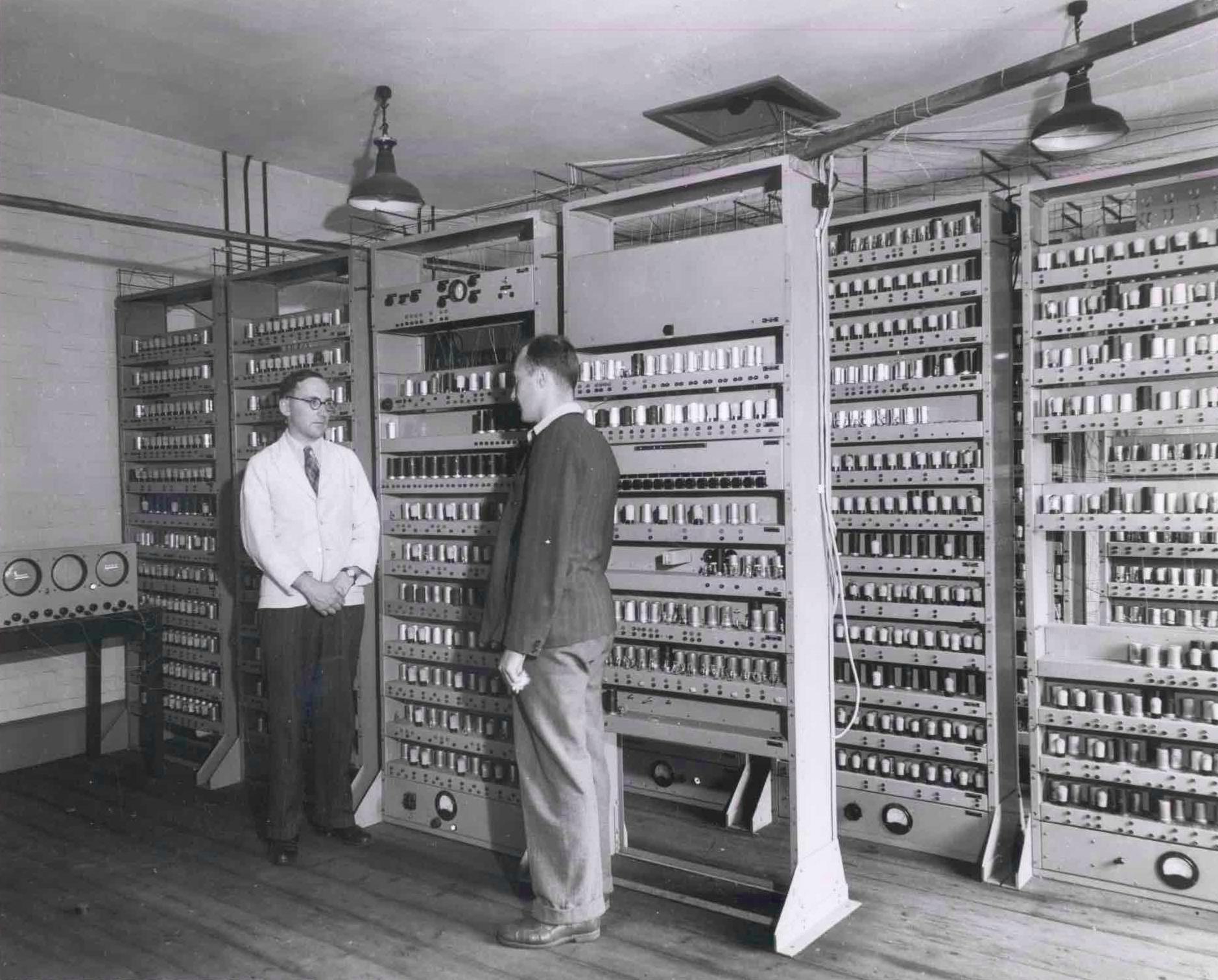
.jpg)
The EDSAC’s store held words consisting of 17 bits. An instruction — an order, in the vocabulary of the time — occupied exactly one such word, divided into four fields:
      5 bits      1        10 bits       1
   ┌───────────┬───────┬──────────────┬────────┐
   │  function │ spare │   address    │ length │
   └───────────┴───────┴──────────────┴────────┘
Here is an example of one such order as a sequence of 17 bits:
   1 1 1 0 0    0    0 0 0 1 0 1 1 0 1 0    0
   ─────────    ─    ───────────────────    ─
    function  spare         address       length
Function 11100, address 0001011010 — 90 in decimal — and a length bit of 0. The order instructs
the machine to add the number held in location 90 to the accumulator. While this is how orders are
represented and understood by the machine, it is not how one wrote programs for EDSAC. A programmer
would write a sequence of characters representing the orders to be executed onto a paper tape that
EDSAC read into its store and then ran. Below is an example program that represents a small routine
that divides by repeated subtraction, leaving the remainder in location 92. The left-hand column
depicts where the order is stored, the middle column is the sequence of characters that encode the
order, and the right column describes what the order does.
 store     order      description
   56      A 90 F     add the number in location 90 into the accumulator
   57      S 91 F     subtract the number in location 91 from the accumulator
   58      E 57 F     if the accumulator is positive, continue at location 57
   59      T 92 F     store the accumulator into location 92 and clear it
While the above structured representation is helpful to understanding the procedure, the actual
program written to the paper tape didn’t contain the store location of instructions, the description
or any white space. The tape would simply read A90FS91FE57FT92F and then relied on being loaded
into the store from location 56 onward.
The description in that third column, and everything else a reader would need, sat outside the tape entirely. What a routine was for lived on its manuscript — a separate sheet, written out by hand, setting out the same orders with commentary beside them. Even the program’s name was kept outside the program: the practice was to write it on the tape in pencil.
The gap between the bits in the store and the characters on the tape is smaller than it appears. A
paper tape records characters as five-bit teleprinter codes, and an order’s function field is five
bits wide — so the order code was numbered to make the two coincide. 11100 is at once the function
code for add and the teleprinter code for the letter A; 01100 is both subtract and the
letter S. The letter punched on the tape was the function field, already in binary, with
nothing to convert. As Martin Campbell-Kelly writes in his
Tutorial Guide to the EDSAC Simulator,
this “simplified the translation of the symbolic program considerably.”
It is an early instance of hardware being shaped around the
convenience of programming: the order code was numbered to suit the notation a person would write on
the tape.
The addresses got no such help, and that is where the difficulty lived. 90, 91, 92, and 57
are absolute store locations, fixed at the moment the routine was written. Suppose you now need one
more order between the ones at 57 and 58. Everything below the insertion shifts down a word: the two
remaining orders move to 59 and 60, and the three numbers this routine works on, held after the
program, move to 91, 92, and 93. So A 90 F, S 91 F, and T 92 F must each have their address
increased by one, by hand, in the listing. The jump E 57 F points backward, to a location before
the insertion, and must be left exactly as it is.
Note which orders those were. The branch is the one you would think to check, and it is the one that turns out to be fine; the arithmetic orders are what broke, because the data moved even though nothing about the arithmetic changed. That is the whole difficulty in one observation, and it is the documented reason the machine’s loading program was rewritten within months of its first run. In Campbell-Kelly’s account, addresses “had to be coded in absolute form: this meant, for example, that if an extra instruction had to be inserted in a program then the addresses in many of the branch instructions would need to be altered. This made program debugging very tedious.”
And the store itself records none of the distinctions you are relying on. An order is a 17-bit word; so is a number. Which words in the store are instructions is settled by which of them the machine is told to execute, and nothing marks a word one way or the other — which was not merely a theoretical point, because the EDSAC had no index registers. To walk along an array in a loop, a program had to reach into its own orders and increment the address field, treating an instruction as arithmetic data because that was the only way to do it.
From here on, each development moves some piece of bookkeeping off the programmer and into the machine, the program, or the notation itself: where an order sits in the store, which routine performs a standard task, which instructions compute an expression, which declaration a name refers to. Each was also resisted by the programmers who had been doing that bookkeeping by hand, for reasons that were generally sound at the time.
Names for places
The EDSAC’s order code had already made the operation symbolic. The next step was to do the same for the address: let a program work out where things ended up, so that a person does not have to.
The machine’s earliest loading program, the initial orders of spring 1949, read the tape and placed orders in the store, converting decimal addresses to binary. It lasted about three months before its limitations — the absolute addresses above, and the difficulty of keeping a library of subroutines when nothing could be moved — became intolerable. Wilkes handed the problem to David Wheeler, then a research student, with the constraint that the replacement fit in 42 orders. Wheeler’s Initial Orders 2, in service by September 1949, is what Campbell-Kelly calls “the forerunner of the modern assembler,” and was celebrated at the time as “the leading example of programming virtuosity.”
Initial Orders 2 introduced named locations. Fifteen words of store, locations 41 to 55, are each named by a letter, and every order on the tape ends with one of those letters. As an order is loaded, the value held in the named location is added to it, and the sum is what goes into the store. This is why programs are loaded from location 56 onward: the fifteen names sit immediately below.
Three of the names have a fixed convention. F names a location holding the constant value 0, so an
order ending in F is stored exactly as written. D names a location holding the constant value 1,
so an order ending in D is stored with its length bit set, which denotes its operand as long.
θ names a location holding the origin of the routine currently being loaded, set by a directive at
the head of each routine. When used, θ makes the address bits of an order relative to the routine’s
start rather than absolute.
  the tape says          loaded at 56          loaded at 200
     A 5 θ          →       A 61          or       A 205
This allows one to write a program and have it be correct no matter which location the program is written to. This is relocation, and it is what makes writing a subroutine library possible: a routine can be written once, by someone with no idea which program will use it or what else will be in the store, and can be stored in any available region of the store.
In addition to the three above names, there are twelve names that by convention can be set by the
programmer before a subroutine is written to the store and used to denote a region of store
locations. For example, a programmer might use the name M to hold the location 90 (where they want
to store their program’s data) and then use M within their program to access data elements without
worrying where exactly that region of data lives within the store. Using these named locations, we
can rewrite the division routine from earlier as follows:
 order       description
 A 0 M       add the number at M+0 into the accumulator
 S 1 M       subtract the number at M+1 from the accumulator
 E 1 θ       if the accumulator is positive, continue at θ+1
 T 2 M       store the accumulator at M+2 and clear it
No absolute location appears anywhere in it. The branch says back to the second order of this
routine rather than back to 57; the operands say the first three words of my data rather than
90, 91, and 92. The routine can now be loaded anywhere. Its data can be moved by changing the one
value held for M, and the arithmetic orders that broke in the earlier version — the ones that broke
because the data had moved rather than because the arithmetic had changed — need no editing at all.
Branches within a routine are not covered. Insert an order ahead of the target and E 1 θ must still
become E 2 θ by hand: the position is relative to the routine, but it is still a position. Code
letters removed the surprising half of the problem and left the half a programmer would think to
check. Removing the rest takes names for the positions themselves — labels, as every assembler since
has had — which the EDSAC never acquired.
The same idea was arriving elsewhere. Kathleen Britten and Andrew Booth’s 1947 report Coding for A.R.C., written for the relay machine they had built at Birkbeck College, is among the earliest documented descriptions of a symbolic notation for a machine’s orders together with the program that translated it. Wilkes, Wheeler, and Gill’s 1951 account of the Cambridge system is both the first programming textbook and the first published description of a library of reusable subroutines.
What this step leaves alone is as important as what it changes. One order on the tape is still one order in the store. The program says, in sequence, what the machine is to do, and a programmer reading it can still predict every instruction that will execute. That correspondence is why the objections to this step were mild, and why the objections to the next one were not.
Automatic programming, and the first serious objection
The abstraction so far has been about where: a code letter stands for a location and the loader works out the number, though a programmer still writes every order that runs. The next step abstracts what. If a loading program can place a subroutine and fix up its addresses, it can also be asked for one by name — write take a square root, and the routine computing it is supplied and fitted in. From here a program is assembled out of routines, and which orders carry them out is settled by the program doing the loading. In 1952 Grace Hopper described a system doing exactly that — the A-0, running on the UNIVAC — in a paper called “The Education of a Computer”. The argument she makes there is about where the labour goes:
This situation remains static until the novelty of inventing programs wears off and degenerates into the dull labor of writing and checking programs. This duty now looms as an imposition on the human brain. Also, with the computer paid for, the cost of programming and the time consumed, comes to the notice of vice-presidents and project directors.
Her conclusion is that the programmer, handed a catalogue of subroutines, “may return to being a mathematician” and “does not even need to know the particular instruction code used by the computer.” The machine assembles the program; the person states the problem.
The objection to this was immediate, widespread, and for the time correct. Writing about the same period, John Backus is blunt about how the systems actually performed: “All of the early ‘automatic programming’ systems were costly to use, since they slowed the machine down by a factor of five or ten.” A factor of five is not a rounding error on a machine whose time is billed by the hour. And the people objecting were not being territorial. Backus’s own summary claims that these positions were justified:
Before 1954 almost all programming was done in machine language or assembly language. Programmers rightly regarded their work as a complex, creative art that required human inventiveness to produce an efficient program.
From that viewpoint, it was efficiency in particular that looked impossible to automate:
Experience with slow “automatic programming” systems, plus their own experience with the problems of organizing loops and address modification, had convinced programmers that efficient programming was something that could not be automated.
Both halves of the debate were grounded in daily experience. The “address modification” mentioned is the problem from earlier in this chapter — a loop over an array rewriting its own orders — and Backus lists the lack of index registers first among the difficulties the computers of that era created. The objection came from people who had been doing that work by hand for years.
So there were two true statements in circulation. Automatic programming produced programs several times slower than a competent person would write. And, as Backus notes elsewhere in the same paper, the cost of the programmers at a computing centre was “usually at least as great as the cost of the computer itself,” with programming and debugging accounting for as much as three quarters of the cost of operating one. Both facts are correct. The disagreement was over which cost dominated, which is an empirical question about the state of the world. As machines got cheaper, programs got larger, and translators got better, the answer moved towards supporting the abstraction Hopper argued for.
Expressions
Fortran began at IBM in 1954, and its name is a contraction of “FORmula TRANslating System.” Backus had proposed the project in a letter to his manager in late 1953, giving the cost of programmers as one of his prime motivations. What it let a program state was a formula:
A + B * C
In the EDSAC orders earlier in this chapter, the sequence of orders is the order of operations:
the programmer decides that the multiplication happens before the addition, finds a location to keep
the product in until the addition needs it, and writes the orders that carry that out. The line
above sequences nothing. It records which operations combine which values, and the translator
derives a sequence from it. For an array element such as A(I,J) it also generates the
arithmetic that turns two subscripts into the single address an instruction can name. Each of those
had been done by hand, in a notebook, and redone after every edit.
The Fortran team understood the objections they were up against, and organized the entire project around answering them rather than around the language. Backus, looking back in 1978:
It was our belief that if FORTRAN, during its first months, were to translate any reasonable “scientific” source program into an object program only half as fast as its hand coded counterpart, then acceptance of our system would be in serious danger. This belief caused us to regard the design of the translator as the real challenge, not the simple task of designing the language.
While the above quote noted that half speed was the point of expected failure, the target for acceptance was much higher: Backus writes that a system of this kind would be widely used only if it could be shown to produce programs “almost as efficient as hand coded ones” and to do so “on virtually every job.” Fortran shipped in 1957 with an optimizing compiler because that target was far beyond anything an automatic system had reached; the earlier ones ran five to ten times slower than hand coding.
The earlier systems’ slowdown had gone mostly into floating-point subroutines, which let those systems get away with crude housekeeping: simulated indexing and loop control cost far less time than the floating-point arithmetic they surrounded. The IBM 704 incorporated hardware instructions for floating-point operations and indexing, speeding the arithmetic up by a factor of ten and, in Backus’s phrase, “leaving inefficiencies nowhere to hide.” The largest component of the old slowdown was gone, and the bookkeeping left over — loops, tests, subscript arithmetic — was now a visible share of the program’s running time.
Generating good code for the 704 was the hard problem, and designing the language looked like the simple part in 1954. The rest of this book is a record of how much was hiding in language design — scope, binding, types, evaluation order, and what a function even is. Backus, writing in 1978, still held that the priority had been the right one: had they failed to produce efficient programs, “the widespread use of languages like FORTRAN would have been seriously delayed.” Later languages could afford to sit further from the instruction set, and to give up more against hand-optimized code, because a translator had already been shown to close that gap.
Fortran I did what it set out to do, and it did it for one machine: the compiler turned formulas
into IBM 704 instructions. However, the formulas that programmers wrote (e.g., A + B * C) were
just arithmetic expressions; which instructions computed them was left to the translator. This is
what later made it possible to run the same program on a different machine, and it is what this
book relies on when it asks what a construct means separately from how it runs.
Structure
Algol 60 arrives at the start of the next decade. The abstractions so far had mechanized the bookkeeping that programmers were already doing. Algol 60 introduced ideas about programs that had no counterpart in machine code, in assembly, or in Fortran I. Hoare, in “Hints on Programming Language Design” thirteen years after the ALGOL 60 report and with no particular reason for flattery, wrote:
The more I ponder the principles of language design, and the techniques which put them into practice, the more is my amazement and admiration of ALGOL 60. Here is a language so far ahead of its time, that it was not only an improvement on its predecessors, but also on nearly all its successors.
Algol’s practical reach was narrower than Fortran’s — scientific and industrial computing ran on Fortran for decades — but the report’s influence on how languages are described and designed is hard to overstate.
Algol 60 introduced block structure: a program has nested regions, and a name declared inside a region means something there and not outside it. On the EDSAC, location 90 was location 90 for the whole run; a code letter held one value at a time, for whoever was loading. There was no notion of a name having a region of validity, because there was nothing for such a region to be made of. Block structure made “where does this name refer to?” a question with a principled answer, determined by the program’s own shape. Part III of this book is spent on that answer and on what it takes to implement it.
The Algol 60 report specified the language’s syntax in a formal notation — what is now called Backus–Naur Form (BNF) — rather than in prose and examples alone. Syntax and semantics picks this up directly; for now the relevant point is that it became possible to ask whether a program belonged to the language, and the answer did not depend on any particular compiler. Algol 60 was defined by an international committee, in a report, before there was a compiler for it. That inverted the previous arrangement, under which a language was whatever the translator happened to accept and the manual described that translator’s behaviour. Once the definition is the document, several implementations can exist and be compared against it, and the question “is this a compiler bug or a program bug?” becomes answerable.
What does it mean to be “high-level”?
The label “high-level” has moved at every step in the history this chapter describes and has not stopped since. Assembly was the automatic programming of 1950 and became the baseline against which Fortran was accused of inefficiency. C was classed among the high-level languages when it took shape in 1972, though Kernighan and Ritchie hedged even then: The C Programming Language (1978) calls it “a relatively ‘low level’ language.” Today the hedge is gone; C is simply a low-level language, and not much about C itself has changed.
The reason is that “high-level” measures a distance from the machine, and both ends of that measurement move: the languages rise, and the machine itself becomes an abstraction. A modern processor’s instruction set is an interface over a microarchitecture that pipelines and reorders instructions, renames registers, predicts branches and speculates past them, and — on a multiprocessor — allows one core to observe another’s writes in an order the program never wrote. Even hand-written assembly no longer says what will physically happen, let alone in what order another core will see it happen. The bottom of the stack is a moving target too.
Which suggests that “how high-level is this language?” is a weaker question than the two it usually stands in for:
- What does this notation let me stop saying? Every step above answers this concretely: addresses, instruction selection, temporaries and evaluation order, the region in which a name is valid.
- What does the language now decide on my behalf, and can I predict what it will decide?
The second question is where every objection in this chapter lived. “It will be five times slower” and “efficient programming cannot be automated” are both versions of I can no longer predict what the machine will do, which in 1954 was the same worry: what the translator decided was exactly which instructions ran. That concern never went away, and it should not: it has only changed granularity. Whether a line allocates, whether a loop will vectorize, when the collector will stop the program, what an optimizing compiler is permitted to assume, which language to write a kernel in — each is the same question asked about a taller stack. What changes is the answer, and the answer depends on facts about hardware, program size, and what people’s time is worth.
How language features come to be
Every abstraction built in the rest of this book arrived by the route just described. Scope, static types, first-class functions, pattern matching, automatic memory management: each was once a proposal that someone had to argue for, against people who could point at a real cost and were not wrong to. By the time an idea reaches a textbook it looks as if it were inevitable, and that appearance hides both how the idea came about and what the alternatives to it were.
When this book introduces a concept, it starts where the concept started: with the problem it solves, the objections raised against it, and the different answers other languages settled on, many of them still in use. Appendix F lays the same material out in date order, for readers who want the arc in one place.
Further reading
Before there were languages: Williams and Kilburn’s letter “Electronic Digital Computers” (Nature, 25 September 1948) runs a few hundred words and announces that a machine in Manchester had been running stored programs for some weeks. That machine is the Manchester Baby, which opens this chapter, and the letter is the first public notice that a program held in a machine’s own memory had actually run. For the machine in detail, including the input device and the surviving text of the first program, see Simon Lavington, A History of Manchester Computers, 2nd ed. (British Computer Society, 1998), and the University of Manchester’s Computer 50 archive. Kathleen Britten and Andrew Booth’s Coding for A.R.C. (1947) is an early written account of a symbolic notation for a machine’s orders and the program that translated it; Britten — later Kathleen Booth — wrote it as a research assistant at Birkbeck College. It is frequently called the first assembly language.
Programming the EDSAC: Cambridge’s EDSAC collection holds the machine’s order code and its operating log, kept by chief engineer W. S. Renwick and transcribed by David Wheeler; the entry for 6 May 1949 reads in full: “Machine in operation for first time. Printed table of squares (0-99), time for programme 2 mins. 35 secs. Four tanks of battery 1 in operation.” Wilkes, Wheeler, and Gill’s The Preparation of Programs for an Electronic Digital Computer (1951) is the first programming textbook and the first published description of a subroutine library: its second half catalogues the EDSAC library subroutines by category, Chapter 7 works through five complete programs, and Chapter 8, “Automatic Programming,” covers assembly, floating addresses, and formula recognition — in 1951. Martin Campbell-Kelly’s Tutorial Guide to the EDSAC Simulator (EDSAC Replica Project, The National Museum of Computing) is the source of the order code and instruction format described above, and comes with a simulator that runs the historical programs and any you write yourself.
Automatic programming and its critics: Grace Hopper’s “The Education of a Computer” (1952) makes the case for automatic programming, argued from the economics of programmer time rather than from elegance. Backus’s “The History of Fortran I, II, and III” (1978, delivered at the first of the HOPL conferences below) records what the objectors said and why they were not being foolish; its opening sections on attitudes toward “automatic programming” and on the economics of programming in the early 1950s are the best short account of why this was a real dispute. For the system as its authors presented it at the time, before it had a history, see “The FORTRAN Automatic Coding System” (1957).
Defining a language: Naur’s “Report on the Algorithmic Language ALGOL 60” (1960) is short and still readable — skim §1 to see a language’s syntax being specified formally for the first time. Hoare’s “Hints on Programming Language Design” (1973) is design advice from the era when designing the language had stopped looking like the simple part, and the annotated reading list in its appendix is a short opinionated bibliography of the field as it stood then.
Designers on their own work, and surveys: Dennis Ritchie’s “The Development of the C Language” (1993) traces C to its BCPL and B lineage and to the PDP-11, a designer describing decisions rather than defending them. It appeared at the second of the History of Programming Languages conferences, whose proceedings — HOPL I (1978), HOPL II (1993), HOPL III (2007), and HOPL IV (2021) — are the standard place to find designers writing the history of their own languages, with the partiality that implies and the detail nobody else could supply. For a survey of the whole field rather than a single language, Jean Sammet’s Programming Languages: History and Fundamentals (Prentice-Hall, 1969) covers more than a hundred languages while most of them were still in use, and records what the field thought it was doing before anyone knew which lines would matter. Donald Knuth and Luis Trabb Pardo’s “The Early Development of Programming Languages” — Encyclopedia of Computer Science and Technology, vol. 7 (1977): 419–493, reprinted in Knuth’s Selected Papers on Computer Languages (CSLI, 2003) — is a systematic survey of the pre-Fortran systems this chapter compresses into a paragraph, including several that were ahead of anything described here but left no descendants.
Concept checks
The EDSAC's function codes were symbolic from the start; its addresses were not. Why did that asymmetry exist, and what did fixing it require?
The function code was free. Numbering the order code so that each function’s bit pattern is the teleprinter code of its letter costs nothing at all — it is a choice about which numbers to assign, made once, and after it the letter on the tape is the function field. An address cannot be handled that way, because its correct value is not known when the order is written: it depends on where the routine ends up in the store and on how many orders precede it, both of which change on every edit.
Fixing it therefore required something the function code did not: a program that computes at load time. Initial Orders 2 added a value to each order as it was placed, so the address could be written relative to an origin fixed later. This is the general shape of the thing — an abstraction is usually a way of writing down information that was previously only in someone’s head, and the ones that are hard are the ones where the information is not available until later.
Programmers in 1954 objected that automatic programming produced code five to ten times slower than hand-coding. Was the objection correct?
Yes, as a description of the systems then available — Backus, who was on the other side of the argument, says so plainly. The objection stopped holding for reasons largely outside the argument: compilers improved, machines got cheaper while programmer salaries did not, and programs grew past the size at which hand-optimizing all of one is possible. There is also a wrinkle in the other direction: the IBM 704’s hardware floating point made translated code’s inefficiency more visible rather than less, by removing the slow subroutines it had been hiding behind. The lesson is that an engineering objection is usually a claim about current conditions, and stays true only as long as the conditions do.
Assembly and Fortran both transfer bookkeeping to the machine. What does Fortran give up that assembly keeps?
Assembly preserves a one-to-one correspondence: one line, one instruction, and a reader can predict exactly what executes. Fortran breaks it. The translator chooses which instructions to emit, where to put temporaries, and how to compute a subscripted address, so the same source can produce different instruction sequences on different compilers or machines — and the program no longer describes any particular machine’s behaviour. That break is what made the efficiency objection serious, and it is also the property that later made the same program runnable elsewhere. The two are the same fact seen from opposite sides.
ALGOL 60 was specified in a committee report before any compiler for it existed. What does that arrangement make possible, and how can it fail?
It makes the language independent of any one implementation: several compilers can exist and be judged against a common definition, disagreements become answerable by citing a document, and “compiler bug” becomes a meaningful accusation. It also makes a language possible to study — the report can be read, criticized, and used as a model, which is most of why ALGOL’s influence outran its use.
The failure mode is specifying something nobody knows how to implement well, or that means less than it appears to. ALGOL 60’s call-by-name parameters are the standard example: cleanly defined in the report, surprising in behaviour, and awkward to compile (Evaluating function calls explores this in detail). A committee writing without an implementation has nothing forcing it to discover the cost of an idea.
"High-level" has been applied to assembly, to Fortran, and to C, and withdrawn from all three. What question is worth asking instead?
Two, both concrete. What does this notation let me stop saying? — addresses, instruction selection, evaluation order, the extent of a name’s meaning; the answer is a list, and lists can be compared across languages. And what does the language now decide for me, and can I predict what it decides? — which is where the real disagreements are, historically and currently. Every objection in this chapter is a version of the second question, and so are modern arguments about garbage collection pauses, undefined behaviour, and what an optimizer may assume. “How high-level is it?” only measures distance from a baseline that keeps moving, in both directions.
The Paradigm Branches
The previous chapter followed a single idea of what a program is. Machine code gave way to assembly, assembly to Fortran and Algol, and each step handed more bookkeeping to the translator — addresses, instruction selection, the region in which a name is valid. What none of those steps touched was the idea underneath: a program is a sequence of commands that change the machine’s state, one after another. Fortran raised the level of the commands and Algol organized them into blocks, but a program was still a list of commands to modify the machine’s store.
That idea is an answer to a question the languages in that chapter never stopped to ask, because the machine answered it for them. The question is: what is a program? The store-and-command picture is one answer, and it is the machine’s own answer, lifted through levels of abstraction; however, there are other notions of what a program is. These notions differ from the store-and-command notion, and from each other, not in how their programs are spelled but in what they take a program to be. This chapter lays out the main answers and the communities that gave them, and marks which part of the book describes each one.
What does it mean to be a program?
The word paradigm entered programming through Robert Floyd’s 1978 Turing Award lecture, which borrowed it from Thomas Kuhn’s account of how a scientific field settles on a shared way of framing its problems. A programming paradigm is that: a shared idea of what a program is and how you go about writing one. Four such ideas organize most of the languages in use, and each can be stated as an answer to what is a program?
A sequence of commands. A program is a list of instructions that read and change a shared, mutable state, carried out in order. This is the imperative view of what a program is. This view derives from the machine’s model of a program, often abstracted to higher-level notation: assigning to a variable, looping, iterating through an array. Each of these operations is about doing something to the state of the program that persists between each step of the program.
Consider the following task: given a set of directed edges and a starting node, which nodes can
be reached? Below is an imperative program that accomplishes this task. The program works by keeping
two pieces of state: a set of nodes already visited, and a frontier of reached nodes whose
outgoing edges it has not yet examined.
visited  = { start }
frontier = [ start ]
while frontier is not empty:
    n = frontier.pop()
    for each edge (n, m):
        if m not in visited:
            visited.add(m)
            frontier.push(m)
return visited
Both visited and frontier hold only the start node in the beginning. Each pass through
the loop takes a node off the frontier, looks at every edge leaving it, and for each target it
has not seen before adds that target to the visited set and pushes it onto the frontier
to examine later. When the frontier is empty, every reachable node has been visited, and
visited is the set of nodes reachable from start.
The application of functions to values. A program is an expression, and running it means
evaluating that expression to a value. There is no store being modified in the background; a name
stands for a value and is not modified. This is the functional view of programming. Its origins
predate any computer, in Alonzo Church’s λ-calculus of the 1930s,
a formalism in which everything is a function and computation is substitution. John McCarthy’s Lisp,
whose eval we discussed previously, was the first functional language, borrowing Church’s notation
for functions if not the whole calculus. Where the imperative program says do this, and update that,
the functional program says the answer is this expression, and leaves the order of evaluation as a
detail.
Below is a functional program for the same graph reachability task. It names the reachable set as the result of growing a set of reached nodes one edge-step at a time, until a step adds nothing more:
step(seen) = seen ∪ { m | n ∈ seen and (n, m) is an edge }

grow(seen) = if step(seen) = seen then seen else grow(step(seen))

grow({ start })
The function step takes a set of nodes reached within n steps and returns a new set with every node
reached within n+1 steps, without modifying the input set. The function grow repeatedly applies step
until the set of seen nodes has reached a fixed point (the same before and after applying the step function).
That stable set of nodes is the answer; it is obtained by evaluating an expression rather than accumulated
by a loop that updates the set of seen nodes.
A set of facts and rules. A program states what is true — these edges exist; a path exists when an edge does, or when a path reaches an edge — and running it means asking what else must be true and letting the system work it out. Nothing in the program says how to search. This is the declarative, or logic, view of programming. It grew out of automated theorem proving in the early 1970s, when Robert Kowalski argued that a piece of logic could be viewed as a program and Alain Colmerauer’s group in Marseille built Prolog around that view. Bridger’s relational sublanguage takes the same idea in a smaller, always-terminating form.
Below we show how the graph reachability task is encoded as a declarative program. The program itself
prescribes no search mechanism; the two clauses state what it means to be reachable from the start node,
and finding the nodes that satisfy the clauses is the system’s job:
reach(start).
reach(Y) :- reach(X), edge(X, Y).
The first clause says the start node is reachable. The second says that if X is reachable and there
is an edge from X to Y, then Y must also be reachable. Nothing names a node to visit first, and no set
is maintained; the program stores no state and describes no procedure. When one asks which nodes are
reachable, the system returns the smallest collection of facts that makes both clauses true.
A society of objects exchanging messages. A program is a collection of objects, each holding some private state and knowing how to respond to requests; computation happens as they send messages to one another. This is the object-oriented view of programming. It appeared in Simula 67, built by Ole-Johan Dahl and Kristen Nygaard to describe simulations in which each entity carries its own state, and was made central by Alan Kay and the Smalltalk group, for whom the messages between objects mattered more than the objects themselves.
Recall the graph reachability task. In the object-oriented program below, the graph becomes a
collection of node objects, each holding its own list of neighbors, and the search happens as the
nodes send one another a reach message:
class Node:
    neighbors                     # the nodes this one points to

    method reach(visited):
        if self ∈ visited: return
        visited.add(self)
        for each n in neighbors:
            n.reach(visited)      # send the same message onward

start.reach({ })
Each node, on receiving reach, records itself in the shared visited set and then sends the same
message to each of its neighbors, which do the same. The visited set both collects the answer and
keeps a node from responding twice, so a cycle does not loop forever. The traversal is the imperative
one from before, redistributed: no central loop drives it, and the work is carried by objects passing
a message along the edges.
What differentiates paradigms
While many imperative programs share similar syntactic forms — and similarly for functional, object-oriented, and declarative programs — the form of a program does not dictate which paradigm it belongs to. The declarative reachability rules could be written in a C-like block syntax, or the imperative worklist algorithm above in Lisp-style s-expressions, without either changing paradigm. What decides the paradigm is what a language treats as primitive and free, and therefore what it lets you leave unsaid.
The imperative program leans on a mutable store as something that is simply there: a variable is a box you can overwrite, and overwriting it costs nothing to express. The functional program has no such box — a name binds to a value and the binding does not change — so anything resembling a running change must be expressed some other way, by producing a new value rather than editing an old one. The declarative program treats search as free: it never says how the answer is found, because supplying the how is the system’s job, not the programmer’s. What one paradigm makes implicit, another makes you spell out.
A consequence is that the paradigm is not a property of a language’s grammar, and one language can host more than one. A programmer can write in a functional style inside an imperative language by refusing to mutate and building with recursion and functions that take other functions as arguments; a programmer can write imperative code inside a functional language wherever it provides a way to. The paradigm a program belongs to is the set of defaults it works with — what it treats as primitive and what it leaves implicit — and a language belongs to a paradigm by making one set of those defaults cheap and the others deliberate.
This is why paradigm fit is something a working programmer can feel. Reachability written imperatively carries a visited set and a worklist that are bookkeeping, present only to drive the search; the same problem written as rules has neither. On the other hand, for a task like a running total over a stream of inputs, or an in-place simulation that updates a grid each tick, the imperative version is succinct, while the declarative framing strains to express a process that is inherently about change over time. The awkwardness comes not from the program being wrong, but from the problem not fitting the strengths of the paradigm it is expressed in.
Multi-paradigm languages
While this chapter names four paradigms, most programming languages let programmers express programs across two or more of the paradigms. Lisp, a typical example of a functional language, had an assignment operator early and has allowed programs with mutable state ever since. In Smalltalk, each method of an object has an imperative body. Most languages a reader is likely to know support multiple paradigms: Python has objects, first-class functions, and imperative loops all at once; Rust, the language this book asks you to write the Bridger interpreter in, has all three as well, and a type discipline over them. Peter Van Roy’s survey of the field catalogues on the order of thirty paradigms once combinations are counted. This is a sign that the paradigms are overlapping views of a program rather than distinct ones: a paradigm is really about the decisions a language makes about what it supports and makes freely available to the programmer.
A paradigm, then, is a language’s center of gravity — the framing it makes cheapest and treats as primitive — and not a strict inability to write programs in a different paradigm. Floyd’s lecture already pointed this way: he treated paradigms as techniques a programmer should collect and move between as the problem demands, rather than allegiances to hold. The taxonomy is worth having for exactly the reason it is worth distrusting: it names real differences in what a language makes easy, while most real languages support multiple paradigms with varying ease.
Bridger’s philosophy
Bridger is built to be multi-paradigm, so every part of this book adds to one language rather than touring several. Keeping the comparison inside a single language is what makes it clean: with one syntax, one evaluator, and one notion of a value, a difference you see between two programs is a difference in the idea rather than an artifact of four separate syntaxes, toolchains, and libraries. One language also lets a single program cross paradigms — building a structure imperatively, querying it relationally, folding the results functionally — which is where the trade-offs stop being abstract. And with every framing within reach, you can feel which one a problem wants: you reach for the one that makes the problem short, and notice when a framing fights you.
The core is imperative and functional together: an expression-oriented language, in which even a loop or an assignment produces a value, with first-class functions and closures on one side and mutable references on the other. Onto that core the book adds a static type discipline, a Datalog-style relational sublanguage for the declarative framing, algebraic data types for modeling structured data, and objects assembled from those data types with methods. Each is introduced where the book reaches it, motivated by the problem it answers and set against the alternatives other languages chose.
Looking ahead
The branches named here are built in the order that lets each rest on the last.
- The imperative core is the subject of Parts II through IV: evaluating expressions to values, binding names in an environment, and then the state and control flow — mutation, conditionals, loops — that make a program a sequence of steps over a store.
- The functional branch arrives in Part V, with first-class functions, closures that capture the environment they were written in, and the recursion and higher-order functions that let a program be built by combining functions rather than by issuing commands.
- The type discipline follows in Part VI, as a pass over the core that analyzes programs before they run and rejects any that would use a value in a way its type forbids.
- The declarative branch is Part VII: relations defined by facts and rules, evaluated by finding the smallest set of facts closed under the rules, and queried from ordinary code.
- Algebraic data types in Part VIII give a precise way to describe structured data and take it apart by pattern matching, and they are the material the last branch is built from.
- The object-oriented branch closes the build in Part IX, as structs carrying state together with the methods that act on them.
The final part sets the branches against one another on shared problems, where choosing the framing that fits is the whole exercise. Appendix F places the languages and ideas named above in date order, each linked to the chapter that takes it up in full.
Further reading
A paradigm as a unit of thought: Robert Floyd’s Turing Award lecture “The Paradigms of Programming” (1979) is where the word, borrowed from Thomas Kuhn’s The Structure of Scientific Revolutions, entered the field. Floyd’s argument is that paradigms are techniques to be identified, taught, and expanded, and that a language should support more than one — the framing this chapter and this book take. Peter Van Roy’s “Programming Paradigms for Dummies: What Every Programmer Should Know” (2009) maps the paradigms against one another by the concepts they add, and reaches roughly thirty once combinations are counted — the concrete form of the claim that the pure cases are the exception.
The functional framing against the imperative default: John Backus’s Turing lecture “Can Programming Be Liberated from the von Neumann Style? A Functional Style and Its Algebra of Programs” (1978) argues that the command-and-store model carried from the hardware is a limit on how programs can be built, names the “von Neumann bottleneck,” and proposes a functional alternative — a designer of Fortran arguing against the style Fortran helped establish. Part V takes up the functional lineage in full.
Logic as a programming language: Robert Kowalski’s “Algorithm = Logic + Control” (1979) makes the case that a program has a logical content, saying what is true, separable from the control that says how to search — the idea under the declarative framing. Alain Colmerauer and Philippe Roussel’s “The birth of Prolog” (HOPL II, 1993) is the account of how that idea became a language.
Objects and the messages between them: Alan Kay’s “The Early History of Smalltalk” (HOPL II, 1993) traces the object-oriented framing from Simula through Smalltalk and argues that the messaging between objects, more than the objects themselves, is the idea that matters. Part IX builds objects from the book’s own data types.
Concept checks
Two languages have nearly identical syntax, yet one is called functional and the other imperative. How is that possible?
Because a paradigm is fixed by what a language treats as primitive and leaves implicit. Give one language a mutable store as a free primitive — a variable is a box you overwrite — and its natural programs change state in place. Give the other only value bindings that do not change, and its natural programs produce new values instead. The two can share a grammar down to the punctuation and still make opposite things cheap to express. Syntax is the changeable surface; the paradigm is in the defaults underneath it.
Reachability was short as two rules and longer as a loop. What, specifically, does the declarative version leave out that the imperative one must include?
The search procedure. The imperative version carries a visited set and a worklist and specifies the order in which nodes are taken up and marked — all of it bookkeeping that exists only to drive the computation, none of it part of what reachability means. The two rules state only the meaning: the start is reachable, and following an edge from a reachable node reaches another. The paradigm treats the search as the system’s responsibility, so the program never mentions it. The imperative paradigm treats the store and the stepping as primitive, so the program is written in terms of them.
Bridger puts every branch into one language instead of teaching four separate languages. What would comparing four separate languages confound, and what is given up by not doing it?
With four languages, any difference you observe between two programs could be the paradigm or it could be one of four syntaxes, four sets of values, four toolchains and standard libraries. Holding all of that fixed and varying only the paradigm is what makes an observed difference attributable to the idea rather than the accident — which is why the whole language is one syntax and one evaluator. What is given up is contact with the real languages as they are actually used, with the mature libraries and idioms that a paradigm accretes in practice; the further-reading pointers and the design-space discussions in each part are where those enter.
Name a language usually placed under one paradigm and a place where it clearly leaves that paradigm. What does the existence of such examples say about the taxonomy?
Lisp is typically considered a functional language, but has had assignment since early in its life; Smalltalk is considered and object-oriented language, but its method bodies are ordinary imperative code; Python is taught with objects but has first-class functions and imperative loops in equal standing. The examples are easy to find because the pure cases are the exception. What they show is that the four headings mark a language’s center of gravity — the framing it makes cheapest — rather than a boundary it stays inside. The taxonomy is worth keeping because it names real differences in what a language makes easy, and worth distrusting because almost every real language combines more than one paradigm.
Syntax and Semantics
A programming language is described in two parts. Its syntax fixes what counts as a program: the
rules that decide whether a string of characters is one at all. Its semantics gives each program
a meaning: what it computes, and how. The two are separable: one meaning can be given more than one
syntax, and one syntax more than one meaning. For example x / y in one language divides the values
as integers and in another as reals. Similarly, within a single language x + y may add two numbers
or concatenate two strings depending on what values x and y store.
When you have a bug in your program, it is either a syntax error — an error caused by misspelling your program: an unmatched parenthesis, a misspelled keyword, an unknown language construct — or a logical error: one that results in a program that behaves in an unexpected or inconsistent way. Syntax errors are typically trivial to detect and relatively easy to fix. Logic errors are harder: the program runs, but does the wrong thing, often in subtle ways. Much of what programmers spend their time on (i.e., testing, debugging, verification) is closing the gap between the program written and the program intended, and all of it rests on being able to say precisely what a program means. That meaning is the focus of this book.
Syntax: what counts as a program
A language’s syntax is the set of rules that decide which strings of characters are programs and what structure each one has: characters grouped into tokens, tokens assembled into a tree. Those rules are given by a grammar — a finite set of productions a mechanical procedure can check a candidate program against, and the same productions a parser follows to recover a program’s structure. Whether a string is a legal program is, once the grammar is fixed, a question with a definite answer.
Two layers hide inside the word syntax. The concrete syntax is the text as written — every
parenthesis, the choice of && over and, the whitespace, the fact that multiplication binds
tighter than addition. The abstract syntax is the structure that remains once those surface
choices have done their one job of disambiguating: a tree commonly referred to as the abstract
syntax tree (AST), which records only how the pieces of a program fit together.
The gap between the concrete and abstract syntax is easiest to see by holding the abstract structure fixed, while varying how that structure is concretely written. These three expressions are spelled by different rules:
x + y (+ x y) x y +
The first is infix, an operator written between its operands, the arrangement most languages inherit
from arithmetic. The second is prefix, the operator first, as in Lisp, where every call takes this
parenthesized form. The third is postfix, the operator last, as in the input to a
reverse-Polish calculator.
Three concrete syntaxes — yet a parser for any of them produces the same abstract structure, an
addition with x and y beneath it, and an evaluator handed that structure cannot tell which
spelling it came from. The surface can be redrawn without disturbing what is underneath, which is
why this book starts at the AST: the structure is where meaning will be assigned, and the
AST is the form the rest of the book works on.
In the decade preceding ALGOL 60, a programming language’s syntax was described the same way as a natural language: in prose, with examples, but ultimately determined by the programs its compiler accepted. The ALGOL 60 report gave the language’s syntax in a formal notation instead — now called Backus–Naur Form — precise enough that whether a string is a legal program became a mechanical question the report itself settled, ahead of and independent of any compiler. Backus had introduced the notation a year earlier for ALGOL 58, whose own report still described its syntax in prose; the 1960 report is where a formal grammar became the definition. Syntax has had a clean formal footing ever since.
Semantics: what a program means
Once a string counts as a program, the question becomes what that program means. Previously, we framed meaning as a mapping from a piece of syntax to a mathematical object — the value an expression evaluates to, or a coarser object such as its type. Formally, that mapping is called the semantics of the programming language. A semantics falls into one of two kinds, based on whether the meaning it assigns can be determined without ever running the program.
A semantics is static when the meaning it assigns can be determined by inspecting the program’s
text alone, without ever running it. For example, determining whether every identifier a program
uses is declared and in scope at each of its uses is a static question
(cf. Part III) that can be answered without ever running the
program on any inputs. Similarly, type checking is normally a static check
(cf. Part VI): whether an operation is
applied to a value of the right kind. Consider writing a program where a number is added to a
function. A parser would happily parse the expression x + f, because at the time of parsing both
x and f are simply names. Type checking, however, would determine that x is a name
representing an integer and f is a function, and thus be able to reject the expression x + f
as nonsense.
A semantics is dynamic when the meaning it assigns can only be determined by executing the program. The quintessential dynamic semantics is the concrete semantics: it traces how concrete inputs flow through the program to produce its concrete outputs. The interpreter you build throughout this book, beginning in Part II, computes exactly this, one construct at a time. When we ask what a program means, we typically mean its concrete semantics. A program can pass every static check and still not be the program we intended — i.e., the program can be well-formed, well-scoped, well-typed, and still compute the wrong answer. Static semantics is useful for confirming a program is well-behaved (as prescribed by the static check), whereas dynamic semantics describes its actual observed behavior.
A notation for meaning
ALGOL 60 gave a program’s syntax a formal notation, but its meaning was still written informally, in prose. The written description of the program’s semantics was ambiguous and allows multiple interpretations and open questions about how a program should behave. For example, should an operand short-circuit and not evaluate the right-hand operand when the left-hand one already decides the result? Does an assignment produce a value, and if so which one? Since prose can leave such questions open, two reasonable implementors can read the same description and produce two disagreeing implementations.
Over the years and decades since ALGOL 60, several notations were developed to give a program’s meaning unambiguously (cf. Program semantics). For evaluating expressions, this book uses the following notation
which can be read as in the environment , the expression evaluates to the value . The environment supplies the value of every name in scope, so a variable can be looked up (cf. Part III). The meaning of an expression is given by rules that tell us how to derive the meaning of an expression from the evaluation of the expression’s sub-expressions. Below we show three example rules in turn. The first rule says that the literal evaluates to itself — as does every literal — regardless of the environment.
The next rule states that the variable evaluates to the value assuming that in the environment the variable is bound to the value .
The final rule states that the sum of two expressions is simply the sum of the evaluation of each of those expressions.
This style of writing rules has deep roots in logic and computer science: that the fact below the line is true exactly when every assumption above the line is true. This style of rules dates back to Gentzen’s work in the 1930s on logic, and it’s been used by computer scientists to define how a program executes since Plotkin in 1981 (operational semantics) and Kahn in 1987 (big-step semantics). Throughout this book, we develop these rules into a full account of Bridger’s concrete semantics.
Does the spelling matter?
How a program is spelled shapes how easily it can be read, written, and understood. Over the years,
concrete forms have converged on shared expectations about meaning: a for loop is read as
iterating over a collection, x := e as updating the value a variable holds, infix + as
arithmetic. A reader draws on those expectations from the spelling alone, before working through
what any rule says. The surface governs what a language makes easy to express and easy to grasp, and
a form that cuts against a reader’s expectations misleads about as readily as a poor name.
This book starts past that point, at the abstract syntax — not because spelling is a cosmetic detail, but because this book’s subject is meaning, and meaning is assigned to a program’s structure rather than its surface syntax. How a language chooses its surface, and how that choice shapes the programs people actually write, is a real question with a study of its own; this book simply begins where meaning does.
Further reading
Giving meaning a formal footing: after BNF gave syntax a formal definition, doing the same for meaning took most of the following decade and produced several styles at once. Glynn Winskel’s The Formal Semantics of Programming Languages: An Introduction (MIT Press, 1993) is an accessible book-length review of those semantics, building each from small example languages. C. A. R. Hoare’s “An Axiomatic Basis for Computer Programming” (1969) is the primary source for one of those styles, reasoning about what a program establishes rather than tracing what it does; the operational style the rule above is written in is developed further in Program semantics.
Whether notation shapes thought: Kenneth Iverson’s Turing Award lecture “Notation as a Tool of Thought” (1980) argues the design-space question from the side that says syntax is far from cosmetic — that a well-chosen notation does part of a programmer’s reasoning for them, using the array notation of APL to make the case.
Concept checks
A program is turned away before it runs because it uses a variable that was never declared. Is that a syntax error or a semantics error?
A semantics error — a static-semantics one, specifically. The program is well-formed as text: the grammar has a production for a variable reference, so the parser accepts it and builds an abstract syntax tree. Nothing about the shape of the program is wrong. What fails is a rule about meaning — that a name must refer to something in scope — which is checked by inspecting the program before it runs. It is easy to lump every error the tool catches up front under “syntax,” but scope and type checking are a form of semantic checks, applied to programs the grammar has already accepted.
The expressions x + y, (+ x y), and x y + are spelled by different rules. What do they share, and why can one evaluator serve all three?
They share their abstract syntax: each parses to the same tree, an addition with x and y as its
operands. Infix, prefix, and postfix are three concrete syntaxes for that one structure. An evaluator
is defined over the tree, not the text, so by the time it runs, the choice of spelling is gone — the
information that distinguished the three was consumed by the parser in recovering the structure. A
new surface syntax for the same language only requires a new parser and can continue using the same
evaluator.
Why do we write the semantics as the rule `E-Add` defined above rather than describing it in English prose?
Because English leaves gaps precisely where meaning is contested. A sentence like “an addition
evaluates its operands and adds them” does not say whether the operands are evaluated left to right,
whether either is skipped, or what happens if one fails — and different implementers will fill those
gaps differently, each thinking their implementation is the correct one. An unambiguous rule like
E-Add fixes this issue: it names both sub-evaluations as premises and the combined result as the
conclusion, with no room left for a reader to differ. That precision is what lets a definition also
serve as a specification an implementation can be checked against.
If a language's surface syntax can be replaced without changing what its programs mean, is syntax merely cosmetic?
It is cosmetic to the meaning — swap infix for prefix and every program computes the same thing —
and isolating exactly that is the job of the syntax/semantics distinction. It is not cosmetic to the
programmer. How a program is spelled governs how easily it can be read, written, and understood,
and concrete forms carry expectations that have converged over time — a for loop reads as
iteration, x := e as updating a variable — so spelling shapes what a reader expects a program to
mean and what is comfortable to write, and what is comfortable to write is what gets written. Two
languages with identical semantics can therefore steer people toward different programs.
The Abstract Syntax Tree
Syntax and semantics separated the abstract structure of a program from
the concrete syntax that disambiguates it: three spellings of an addition collapse to one tree.
In this chapter, we detail the concrete implementation of the AST structure of Bridger programs
that the parser provided with this book will have you use in the implementation Milestones.
Specifically, this chapter details three Rust types: Expr for the expressions at the core of
Bridger, Program for whole top-level declarations, and Ty for expressing types. For
complete details on the concrete syntax of Bridger see
Appendix B: concrete syntax.
The shape of expressions
Run down the grammar and an expression is always one of a fixed set of shapes: a literal, a
variable, an operator applied to smaller expressions, a conditional, a call, and so on. A type whose
values are “one of the following” is a sum type, and in Rust it is written as an enum: one
variant per shape, each carrying exactly the pieces that shape is built from. The productions of a
grammar and the variants of a sum type line up one for one, which is what makes the enum the
natural representation of an AST.
That correspondence is old enough to have shaped which languages interpreters get written in.
McCarthy’s LISP (1960) represented programs as the very
lists the language processed — code as data — so a function that transformed a program was an
ordinary list-processing function. The ML family later made the shapes explicit as algebraic data
types and took them apart with pattern matching, a fit close enough that interpreters and
compilers have been written in ML-family languages ever since. Rust inherits both halves: the enum
names the shapes, and match (below) takes them apart.
A tree records structure and drops the surface detail the parser has already used up — the
parentheses, the whitespace, the fact that * binds tighter than +. What survives is how the
pieces fit together, and that is what the type below captures.
Bridger’s Expressions in Rust
The core of Bridger’s syntax is made up of recursively constructable expressions. This section details the components that make up such expressions and how the Book’s companion parser represents the expressions it parses. For convenience in error reporting, every parsed expression includes a span which records where in the source text the expression is located.
struct Span { src: SrcId, start: usize, end: usize }The src says which loaded source the bytes belong to — the prelude is one source and the
program another — so a span names a node uniquely even across files.
A Literal is represented by the following Lit enum. A numeric literal is represented as a
64-bit signed integer in Rust (i.e., all numeric values in Bridger are between and
); a Boolean literal is simply a Rust bool type; a string literal is simply a
Rust String, and a unit literal is the singleton value () left implicit in the Lit enum.
enum Lit { Int(i64), Bool(bool), Str(String), Unit }Before detailing how we represent expressions, we detail several auxiliary types. The enum
UnOp represents all unary operators in Bridger. Similarly, BinOp all binary operators.
Finally, all names (identifiers and variables) are represented as a String.
enum UnOp { Neg, Not, Ref, Deref }

enum BinOp {
    Add, Sub, Mul, Div, Mod,      // arithmetic
    Eq, Ne, Lt, Le, Gt, Ge,       // comparison
    And, Or,                      // boolean
    Concat,                       // ++
    Cons,                         // ::  (prepend to a list)
}

type Name = String;
With each of the auxiliary data types defined, we represent Bridger expressions
with the recursive enum Expr.
enum Expr {
    // a literal value: 5, true, "hi", ()
    Lit(Lit, Span),
    // a variable reference, or the receiver `self`
    Var(Name, Span),
    // a prefix operator: -e, not e, ref e, deref e
    Unary(UnOp, Box<Expr>, Span),
    // a binary operator: e + e, e == e, e and e, e ++ e, e :: e
    Binary(BinOp, Box<Expr>, Box<Expr>, Span),
    // a conditional: if e { … } else { … }, the else optional
    If(Box<Expr>, Box<Expr>, Option<Box<Expr>>, Span),
    // a block: statements and an optional trailing value
    Block(Vec<Stmt>, Option<Box<Expr>>, Span),
    // assignment through a reference: e := e
    Assign(Box<Expr>, Box<Expr>, Span),
    // a function call: e(e, …)
    Call(Box<Expr>, Vec<Expr>, Span),
    // a method call: e.m(e, …)
    Method(Box<Expr>, Name, Vec<Expr>, Span),
    // a lambda: |x, …| e, each parameter optionally annotated x: T
    Lambda(Vec<LambdaParam>, Box<Expr>, Span),
    // a pattern match: match e { arm, … }
    Match(Box<Expr>, Vec<Arm>, Span),
    // a while loop: while e { … }
    While(Box<Expr>, Box<Expr>, Span),
    // a for loop over a list: for x in e { … }
    For(Name, Box<Expr>, Box<Expr>, Span),
    // a for loop over a relation's solutions: for R(a, ?x) { … }
    ForQuery(Query, Box<Expr>, Span),
    // an early return from a function: return e
    Return(Box<Expr>, Span),
    // error propagation: e?  (sugar over match and return)
    Try(Box<Expr>, Span),
    // a tuple: (e, e, …), two or more elements
    Tuple(Vec<Expr>, Span),
    // a list: [e, …]
    List(Vec<Expr>, Span),
    // struct field access: e.f
    Field(Box<Expr>, Name, Span),
    // tuple projection by index: e.0
    Proj(Box<Expr>, u32, Span),
    // constructor application: C(e, …)
    Ctor(Name, Vec<Expr>, Span),
    // struct literal: S { f: e, … }
    Struct(Name, Vec<(Name, Expr)>, Span),
    // a relations operation: add q / clear R / solutions q / query
    Relation(Rel, Span),
}
The comment on each variant names the Bridger form it holds, and every variant matches the abstract
syntax fixed in the language reference. This chapter settles the
shape of each; the chapters that follow give each its meaning. Several variants hold companion
types — Stmt, Arm, Pattern, Rel, and Query — which we define after two structural choices
in Expr itself.
Children sit behind Box. An Expr can contain an Expr (e.g., the two operands of a Binary
operator or the condition and branches of an If) so its size would depend on itself, and no fixed
size would satisfy the Rust compiler. We use Box<Expr> (a pointer to an Expr). Since a pointer
has a known size, a Box<Expr> can be used to hold sub-expressions recursively. A node owns its
children through the Box, and dropping a tree drops everything under it. Where a node has any
number of children — a Call’s arguments, a List’s elements — a Vec<Expr> owns all of them.
Four variants hold companion types, which we define now. A block (Block) is a sequence of
statements followed by an optional result expression, and each statement (Stmt) is either a local
let binding or an expression evaluated for its effect. A ref x = e binding is stored as an
ordinary let of a ref expression, so it needs no case of its own.
enum Stmt {
    Let(Name, Option<Ty>, Expr, Span),   // let x = e   (or   let x: T = e)
    Expr(Expr),                          // an expression evaluated for effect
}
A match expression holds a list of arms. An arm (Arm) pairs a pattern with an optional guard and
the expression to evaluate when the arm is chosen.
struct Arm {
    pat: Pattern,          // the pattern this arm matches
    guard: Option<Expr>,   // an optional `if` guard
    body: Expr,            // evaluated when the arm is taken
}
A pattern (Pattern) describes the shape a match tests a value against, and mirrors the
expression forms it takes apart. Like an expression, every pattern carries its span.
enum Pattern {
    Wild(Span),                                 // _
    Lit(Lit, Span),                             // a literal: 5, true, "hi"
    Var(Name, Span),                            // binds the matched value to a name
    Ctor(Name, Vec<Pattern>, Span),             // a constructor: C(p, …)
    Tuple(Vec<Pattern>, Span),                  // (p, p, …), two or more
    List(Vec<Pattern>, Option<Name>, Span),     // [p, …], with an optional ...rest
    Cons(Box<Pattern>, Box<Pattern>, Span),     // head :: tail
    Struct(Name, Vec<(Name, Pattern)>, Span),   // S { f: p, … }
    Or(Box<Pattern>, Box<Pattern>, Span),       // p | p
}
The relations sublanguage folds its four expression forms into Rel. A query (Query) names a
relation and supplies arguments; each argument (QArg) is either an ordinary expression or a hole
to solve for, named ?x or anonymous ?.
enum Rel {
    Add(Query),        // add R(a, …)
    Clear(Name),       // clear R
    Solutions(Query),  // solutions R(a, …)
    Query(Query),      // a bare query R(a, …)
}

struct Query { name: Name, args: Vec<QArg> }   // R(a, …)

enum QArg {
    Expr(Expr),          // a ground argument
    Hole(Option<Name>),  // a hole: ?x (named) or ? (anonymous)
}
The program that holds them
An Expr builds the core of Bridger’s structure; however, at the top-level, a Bridger program
is a sequence of declarations: functions, globals, types, structs, traits, relations. The
order of declarations does not matter, instead every declaration is visible to every other
top-level declaration (with a requirement that all global names must be unique). As such,
we represent the top level Declarations simply as a map from names to declarations, and
separate trait implementations and rules which are unnamed.
struct Program {
    decls: HashMap<Name, Decl>,   // fn, global, type, struct, trait, relation
    spans: HashMap<Name, Span>,   // where each declaration was written
    impls: Vec<Impl>,             // anonymous: keyed by the type they extend
    rules: Vec<Rule>,             // any number define one relation
}

enum Decl {
    Fn(Generics, Vec<Param>, Ty, Box<Expr>),   // fn f<T: C>(x: T, …) -> T = e
    Global(Option<Ty>, Box<Expr>),             // let x = e  (or  let x: T = e)
    Type(Generics, Vec<Variant>),              // type T<U> = C(U, …) | …
    Struct(Generics, Vec<Field>),              // struct S<T> { f: T, … }
    Trait(Generics, Vec<Sig>),                 // trait Tr<T> { fn m(…); … }
    Relation(Vec<Ty>),                         // relation R : (T, …)
}
The generic-bearing forms — Fn, Type, Struct, Trait, and the impl blocks — each carry a
Generics: a declaration can be parameterized by types, and a type parameter may carry a trait
bound its argument must satisfy:
struct Generics { params: Vec<TyParam> }   // <T, U: Show, …>; empty if absent

struct TyParam {
    name: Name,               // T
    bound: Option<TraitRef>,  // : Show — the trait bound, if any
    span: Span,               // where it is written, for diagnostics
}
The type checker in Part VI reads them — it quantifies a declaration over its parameters, then at each use instantiates them and checks the bound — while the evaluator ignores them, since running the program is type-erased. The reference’s abstract syntax folds them into a note for the same reason; the AST the parser builds keeps them for the checker.
Every Decl bottoms out in Expr — a function’s body, a global’s initializer — so the tree the
last section built is what these hold. Two forms carry no single name and stay out of the map: an
impl is found by the type it extends rather than a name, and a relation is defined by any number
of rules at once, so each keeps its own list. We define the companion types these declarations
use — Param, Field, Variant, Sig, Method, Impl, TraitRef, and the rule forms — below.
Looking a name up is then a map lookup, and that lookup is the order-free, mutually visible scope the reference specifies made concrete: where a declaration sits in the file cannot matter, because the file order is gone once the map is built, and a name declared twice collides when the map is.
A parameter (Param) and a struct field (Field) are each a name with a type, and a constructor of
a type declaration is a variant (Variant) with a name and the types of its fields. Each carries
the span of its own text, so a diagnostic can point at one parameter of a signature. A lambda’s
parameter (LambdaParam) differs from a function’s in one respect: its annotation is optional,
because the type checker can usually infer it from how the lambda is used.
struct Param       { name: Name, ty: Ty, span: Span }            // x: T
struct LambdaParam { name: Name, ty: Option<Ty>, span: Span }    // x  or  x: T
struct Field       { name: Name, ty: Ty, span: Span }            // f: T
struct Variant     { name: Name, fields: Vec<Ty>, span: Span }   // C(T, …), or C
A trait lists method signatures (Sig); an impl supplies methods (Method), which are
signatures with a body. Each records whether the method takes self, its remaining parameters, and
its return type.
struct Sig {
    name: Name,
    has_self: bool,       // whether the method takes `self`
    params: Vec<Param>,
    ret: Ty,              // (), when the return type is omitted
    span: Span,
}

struct Method {           // a Sig with a body
    name: Name,
    has_self: bool,
    params: Vec<Param>,
    ret: Ty,
    body: Expr,
    span: Span,
    sig: Span,            // the signature alone, `fn m(self, x: Int) -> T`
}
An impl block (Impl) records its own generics, the trait it implements if any, the type it
extends, and its methods. A trait named there is a TraitRef — a trait name with any type
arguments.
struct Impl {
    generics: Generics,        // impl<T> …
    trait_: Option<TraitRef>,  // the trait implemented, if any
    ty: Ty,                    // the type being extended
    methods: Vec<Method>,
    span: Span,
    head: Span,                // the header, `impl<T> Tr for T`
}

struct TraitRef { name: Name, args: Vec<Ty>, span: Span }   // Tr, or Tr<T, …>
A rule (Rule) has a head atom and a body. The head (Atom) names a relation and lists its
terms (Term), each a logic variable or a literal. The body is the rule’s and-chain split into
its conjuncts, and each conjunct is an ordinary expression: edge(x, y) and is_ok(x) are the
same syntax, and which of them joins against a relation and which tests already-bound variables
is settled by name resolution when the rules are installed, in Part VII.
struct Rule { head: Atom, body: Vec<Expr>, span: Span }   // rule H :- B1 and …

struct Atom { name: Name, terms: Vec<Term>, span: Span }  // R(t, …)

enum Term {
    Var(Name),   // a logic variable (a lowercase name)
    Lit(Lit),    // a literal
}
The type language
A type annotation on a let, the signature of a function, the fields of a struct, the columns of a
relation, and the bound on a type parameter are all written in one small language of types, and
it is a tree of its own:
struct Ty { kind: TyKind, span: Option<Span> }   // a shape, and where it was written

enum TyKind {
    Int, Bool, Str, Unit,    // Int, Bool, String, ()
    Tuple(Rc<[Ty]>),         // (T, U, …) — two or more
    List(Rc<Ty>),            // [T]
    Fn(Rc<[Ty]>, Rc<Ty>),    // fn(T, …) -> T
    Ref(Rc<Ty>),             // ref<T>
    SelfTy,                  // Self, in a trait or impl
    Named(Name, Rc<[Ty]>),   // N, or N<T, …> when applied
    Meta(u32),               // a type not yet known; the checker solves it (Part VI)
}
The children sit behind Rc, a reference-counted pointer, where the expression tree uses Box.
Types are shared far more than expressions are: the checker records a type for every
expression, nested expressions have nested types, and with plain boxes each level would hold its
own copy of everything below it. With Rc the copies are pointers, and cloning a type costs
nothing.
A type is used in two ways, and the split into Ty and TyKind serves both. A type the
programmer wrote has a position, and a diagnostic can then say that a function was declared to
return Int here and point at the annotation. A type the checker computes has none, so the span
is optional. Two types are equal when their shapes are, wherever they came from, so a Ty compares
and prints as its TyKind alone; Ty::int(), Ty::list(t) and their kin build the computed ones.
TyKind is recursive for the same reason Expr is — a list of a list, a function returning a
function. Named covers both a plain type name and a generic one applied to arguments, with an
empty argument list for the plain case. This is the language the
type checker in Part VI works over; here it is only the shape the
parser records
from a written type.
Matching over the tree
A function over an AST is a case analysis: one arm per variant, handling the pieces that variant
carries. match is Rust’s tool for it, and pulling a node apart binds its fields in the same
motion:
fn depth(e: &Expr) -> usize {
    match e {
        Expr::Lit(..) | Expr::Var(..) => 1,
        Expr::Unary(_, inner, _) => 1 + depth(inner),
        Expr::Binary(_, l, r, _) => {
            1 + depth(l).max(depth(r))
        }
        Expr::If(c, t, e, _) => {
            let branches = match e {
                Some(els) => depth(t).max(depth(els)),
                None => depth(t),
            };
            1 + depth(c).max(branches)
        }
        _ => 1, // remaining forms: Part II onward
    }
}
The recursion in the type becomes recursion in the function, and the shape of each arm is dictated
by the shape of its variant. match is also exhaustive: drop the _ arm and the compiler names
every variant still unhandled, so a new form added to Expr cannot silently fall through a pass
that predates it. That guarantee — the type system enforcing that every case is considered — is why
tree-walking interpreters read so cleanly in this style, and it is the single most useful piece of
Rust for the chapters ahead.
The trees a compiler keeps
The AST here is shaped for a book that walks it directly. A production compiler keeps different trees, and the differences are worth knowing so the choices above read as choices.
A compiler usually holds more than one tree. This one is untyped: it is the parser’s output, and
nothing in it records what an expression’s type is. Part VI’s type
checker leaves the tree as it is and records each
expression’s type in a side table keyed by the expression’s span — which is why a span must name a
node uniquely — so a later stage can consult a type without recomputing it. Names, kept here as
String, are often interned to small integers so that comparing two of them is one machine
instruction rather than a character-by-character scan. And a tree stored with
Box scatters its nodes across the heap; a compiler that cares about locality keeps them in an
arena — one contiguous block — and replaces every Box<Expr> with an integer NodeId index
into it, which also lets the side tables (types, uses) key off a small integer rather than a
span. Each of these buys speed or a place to hang more information, at the cost of a tree that
is heavier to build and read. A first interpreter wants neither cost, so it takes the Box, the
String, and the one untyped tree.
Further reading
Building an interpreter around an AST: Robert Nystrom’s Crafting Interpreters (free online) builds two interpreters for the same language, the first a tree-walker over an AST much like this one, and it is unusually concrete about the shape of the tree and the walk over it. Its “Representing Code” and “Evaluating Expressions” chapters cover the same ground as this one and the next, in Java rather than Rust.
The trees a compiler keeps instead: Andrew Appel’s Modern Compiler Implementation in ML (Cambridge University Press, 1998) develops the typed and lowered intermediate representations named in the last section — separate trees for parsing, type checking, and code generation — and shows what each stage reads off the tree the stage before it produced.
Concept checks
In x + y * z, which variant is at the root of the tree, and why isn't it the + that appears first in the text?
The root is the Binary(Add, …), with x as its left child and the Binary(Mul, …) for y * z as
its right. It is not rooted at the first operator read, because the root is the operator applied
last when the expression is evaluated, and * binds tighter than +. Precedence is a
concrete-syntax rule; the parser has already used it to decide the grouping, and the tree records
only the result. The same tree would come back from (x) + (y * z) or a prefix (+ x (* y z)) —
the surface that distinguished them is gone by the time there is an Expr.
Why does Binary hold Box<Expr> for its operands rather than Expr?
Because Expr is recursive: a Binary contains two Exprs, each of which might itself be a
Binary, with no bound on the nesting. If the operands were stored inline as Expr, the size of an
Expr would include the size of an Expr, and no finite size satisfies that. A Box<Expr> is a
pointer to an Expr allocated elsewhere; a pointer has a fixed size regardless of how large the
subtree behind it is, so the type is well-sized and the recursion lives in the heap rather than in
the type’s layout.
Every variant carries a Span. What breaks if only the root of the tree kept one?
Any node can be the one a later pass needs to complain about — a type error is usually at some operator deep in the tree, an unbound variable at a single leaf — and a diagnostic can only underline what it has a span for. With a span only at the root, every error would point at the whole program. The information is available for free while the parser still knows the offsets, and unrecoverable once the text is gone, so it is recorded on every node even though most nodes never end up in a message.
An arena representation replaces every Box<Expr> with a NodeId index into one array of nodes. What does that buy, and what does it cost?
It buys locality and shared bookkeeping. The nodes sit in one contiguous block instead of scattered
across the heap, which a walk traverses faster, and a NodeId is a plain integer, so side tables —
the type of each node, its uses, its span — can be separate arrays keyed by the same id, letting a
pass attach information to a node without changing the node’s type. It costs directness: reaching a
child is now an array lookup through the arena rather than following a pointer the node owns, the
arena has to be threaded through every function that touches the tree, and Rust’s ownership no
longer frees a subtree for you when its parent goes away. A tree-walking interpreter gains nothing
from the trade, which is why this one keeps the Box.
The top-level declarations are held in a HashMap<Name, Decl> rather than a Vec<Decl> in source order. What decision in the language forces that, and what would a Vec fail to capture?
The language reference fixes the top level as a set: declarations may appear in any order, each is
visible to every other, and a name is declared at most once. A Vec<Decl> would keep the source
order — information the language treats as meaningless — and would let the same name appear twice
without complaint, which the language forbids. A map keyed by name discards the order the language
does not use and turns a duplicate name into a collision when the map is built, so it admits
exactly the programs the reference allows. The impls and rules, which are not singly
named, are the exception the two side lists handle.
Values and Runtime Errors
In the previous chapter, we covered the AST of Bridger as provided by
the accompanying Rust parser. The provided code base also includes a Rust enum type Value
representing the possible values a Bridger expression may evaluate to. Throughout this book,
you will work through the milestones to create an interpreter that evaluates an Expr (and whole
programs) to a Value. This chapter details the Value type you will be working with. It also
covers what the interpreter should produce when an expression has no value at all (a runtime
error). The mathematical value grammar and the semantic rules that define the meaning of Bridger
programs are detailed in Appendix D: language reference.
The space of values
Evaluation produces a value, and every value a Bridger program can compute is one of a fixed set of shapes: an integer, a boolean, a string, unit; a tuple or a list built from smaller values; a constructor value or a struct value; a location into the store; a closure. The reference writes the set as a grammar:
The last two stand for names rather than data — a declared relation, and a struct or type named as the receiver of an associated call — and nothing compares, prints, or stores them.
The above set of values represents the result of running any Bridger program or expression to completion. We describe each in detail in future chapters: integers, booleans, and strings in the tree-walking evaluation as the result of evaluating simple arithmetic, boolean, and string expressions; tuples and lists in that same chapter, as compound expressions built from smaller values; unit, the value of statements and blocks, with control flow; locations with mutable references; closures with functions; and constructor and struct values with algebraic data types and structs later still.
Bridger’s values in Rust
The set of value shapes is a sum type, the same correspondence the AST turned on: one variant per
shape, each carrying what that shape is built from. The Value enum, provided with this book
alongside the AST, holds them. It reuses type Name = String from the
AST chapter for the names in Ctor and Struct.
enum Value {
    Int(i64),                          // 5
    Bool(bool),                        // true
    Str(Rc<str>),                      // "hi"
    Unit,                              // ()
    Tuple(Rc<[Value]>),                // (v, v, …), two or more
    List(List),                        // [] or a cons cell v :: v, see below
    Ctor(Name, Rc<[Value]>),           // a constructor value: C(v, …)
    Struct(Name, Rc<[(Name, Value)]>), // a struct value: S { f = v, … }
    Ref(Loc),                          // a location in the store (Part IV)
    Closure(Rc<Closure>),              // a function + its captured env (Part V)
    Relation(Name),                    // a declared relation, by name (Part VII)
    Type(Name),                        // a type name, receiver of `T.m()` (Part IX)
}
The comment on each variant gives an example of the kind of value it holds, and the variants line up
with the grammar above one for one. The string, tuple, constructor, and struct payloads sit behind
Rc, as the types in the AST chapter do: a value is copied whenever it is
read from a variable or a cell, and a reference-counted pointer makes that copy a pointer bump
rather than a walk of the payload. The Value enum is to a running program what Expr is to a
parsed one: the type every part of the interpreter agrees on for the thing it passes around. Where
Expr is what the evaluator takes apart, Value is what it builds.
One representation choice is visible in List. The reference models a list as either the empty list
or a cons , a head joined to a tail, and the List type holds exactly that: the
empty list, or a cell with a head, a tail, and the length so far, the tail shared with any other
list that ends the same way. Sharing is what makes the rules’ shape a good representation and
not only a good notation. Prepending with ::, taking a list apart with the pattern h :: t,
and head and tail each touch one cell, whatever the list’s length, so a function that
recurses down a list does work proportional to the list. An array would make ::, tail, and
the tail of h :: t copy the whole list. A list literal and ++ cost the left operand’s length,
since its cells are rebuilt onto the shared right operand, and len reads the count each cell
stores. What the array would give back, reading the nth element in one step, Bridger has no
operation for.
Expressions that do not evaluate to a value
Evaluating an expression usually produces a value; however, there are two scenarios when an
expression does not evaluate to a value. Evaluation can get stuck: adding a boolean to an integer,
applying a value that is not a function, projecting a field off a tuple, or dividing by zero. Each
such scenario has no corresponding evaluation rule (and the expression has no well-formed meaning
as a value). Instead, the interpreter immediately halts on such runtime errors. On the other hand,
an evaluation can choose to return early: a return e computes e and then abandons the rest
of the enclosing function’s body, carrying that value out to the function’s own result. We represent
both non-local exits with one type Control in our Rust interpreter.
enum Control {
    Raise(RuntimeError),  // stuck: no rule applies; the run halts
    Return(Value),        // an early return, sent to the enclosing function
}
This chapter describes the purpose of Raise in detail. Stuckness is the absence of a result rather
than a special result, a notion the operational semantics the book writes its rules in makes precise,
and the reference collects the
full list of cases. In the untyped evaluator of Parts II through V, these stuck states are how a
nonsensical program fails; they are Bridger’s runtime errors. Return carries a value that
did finish computing, only not here; a return is legal only inside a function body. We will explain
how return e and the Control::Return variant are treated within the interpreter we build
in the Control flow chapter
and functions.
The interpreter we build must handle expressions that may contain runtime errors. Rather than
having our interpreter crash or have undefined behavior on runtime errors, we have the interpreter
we build make use of Rust’s Result and Error types to represent such runtime errors explicitly.
That means, when the interpreter encounters such runtime errors, rather than halting it stops
evaluation early and returns a RuntimeError describing why the interpreter stopped evaluation.
The variants below are the ones the arms of this part and the next raise; the driver and the
prelude add theirs (no main, a cycle among global initializers, a failed read from input, a
range or a call depth past the machine’s bound, printing a function), and each later part its
own as its constructs arrive (a missing struct field, a method with no receiver, a query inside a
filter).
enum RuntimeError {
    // x not in scope
    UnboundVariable { name: Name, span: Span },
    // 1 + true, a non-bool condition, iterating a non-list, …
    TypeError { expected: Ty, found: Ty, span: Span },
    // 5 / 0 or 5 % 0
    DivByZero { span: Span },
    // .f a value lacks
    NoSuchField { field: String, span: Span },
    // applying a non-function
    NotAFunction { found: Ty, span: Span },
    // wrong number of arguments
    ArityMismatch { expected: usize, found: usize, span: Span },
    // no arm matched the value
    NonExhaustiveMatch { span: Span },
    // == on a function or relation
    NotComparable { found: Ty, span: Span },
}
Evaluation therefore does not return a bare Value. It returns a Value or a Control, and Rust
spells “one or the other” with its own sum type, Result. Its companion Option spells “a value or
nothing”:
enum Result<T, E> { Ok(T), Err(E) }   // a T, or an error E
enum Option<T>    { None, Some(T) }   // a T, or nothing
Both come from Rust’s standard library, and both are how a Rust program carries the possibility of
failure in a value the compiler forces every caller to look at. The evaluator puts a Value on the
Ok side and a Control on the Err side — a normal value, or one of the two non-local exits:
fn eval(e: &Expr) -> Result<Value, Control> {
    match e {
        Expr::Lit(Lit::Int(n), _) => Ok(Value::Int(*n)),
        Expr::Binary(BinOp::Add, l, r, span) => {
            let a = eval(l)?;                 // a Raise or Return bubbles out here
            let b = eval(r)?;
            match (a, b) {
                (Value::Int(x), Value::Int(y)) => Ok(Value::Int(x.wrapping_add(y))),
                (a, b) => {
                    let found =
                        if matches!(a, Value::Int(_)) { type_of(&b) }
                        else { type_of(&a) };
                    Err(Control::Raise(RuntimeError::TypeError {
                        expected: Ty::int(), found, span: *span,
                    }))
                }
            }
        }
        _ => todo!("the remaining forms: the next chapter"),
    }
}
The Ok/Err split names both outcomes at the type level: a caller of eval cannot use the value
without first deciding what to do when it is an Err. The ? after eval(l) is Rust’s propagation
operator — when the subexpression is an Err, ? returns it from eval at once, so whichever exit
it carries — a Raise with its span, or a Return with its value — travels out through every
enclosing operation untouched. One mechanism threads both: every operation propagates a Control
the same way, and only a function call inspects a Return, catching it at the boundary and turning
it back into the call’s value. When both operands are integers the addition proceeds; when they are
not, the last arm raises a RuntimeError::TypeError naming the Ty it expected and the Ty
type_of read from the offending operand, and carrying the addition’s span. The addition wraps,
since the reference fixes integers as 64-bit values with arithmetic modulo .
Two kinds of failure
The Err(Control::Raise(…)) an addition returns and a Bridger value like Err("file not found")
read alike on the page and are different in kind. The first is the interpreter stopping: no rule
applied, so there is no value, and the host Result carries that fact out to the top level, where
it is printed. A Bridger program cannot observe it or recover from it; the program has already
stopped.
The second is an ordinary Bridger value, a constructor value Err(s) that a successful evaluation
produced, which the program inspects with match and carries on from. Evaluating it is a completed
derivation that yields a value; nothing is stuck.
Bridger has its own Option and Result for exactly this second kind of failure, defined in the
prelude as ordinary data types and handled with match — separate from
Rust’s Option and Result, which are how the interpreter is written. The recoverable failures a
Bridger program models with those values, the surface that makes them convenient, and the design
space of failure mechanisms (values against exceptions against a halting panic) are the subject of
Error handling, once
algebraic data types give the language the constructors
to build them. What this chapter fixes is the boundary: a runtime type error is the host stopping,
and it stays outside the values a program computes with.
That boundary is why every stuck case is stated precisely. Each carries a
span and names the Ty it expected against the one it found, because for Parts II through V a runtime
type error is the only report a mistake gets, and the reader debugging a program has nothing else to
go on. When
the type checker arrives in Part VI
it rules out the type-shaped stuck cases before the program runs, trading the clear failures
described here for a guarantee made ahead of time. Division by zero, a failed read from input, and
the interpreter’s two bounds — on call depth and on the size of a range — cannot be ruled out
statically, nor, until exhaustiveness checking arrives, can a match no arm covers.
How a value is represented
A tagged union is one way to give an interpreter a single value type, and the choice reads as a choice against the alternatives a faster or a more open interpreter reaches for.
The enum stores a tag — which variant this is — beside the payload, and every value costs the
tag plus room for the largest variant. match reads the tag to choose an arm, and the compiler
checks that the arms cover every variant, the same exhaustiveness the AST walk relied on. A value
kind cannot be added without editing the one enum and revisiting the matches the addition now
leaves incomplete.
Other interpreters and compilers optimizing for speed instead often make use of smaller, packed value representations. For instance, a production virtual machine for a dynamic language often stores every value in a single 64-bit word, reading a few spare bits as the tag: small integers are represented inline with a tag bit set. This is how OCaml represents its values. It represents its native integers with 63 bits and the low bit determines whether the 64-bit word is an integer or a pointer to a structure. These packed representations achieve faster computations due to the denser representation that leads to fewer memory reads. However, the cost is that the representation is tied to a specific word size, and such packed representations are often hard to read and understand.
An interpreter written in an object-oriented language reaches instead for a class hierarchy: each
value kind a subclass of a common value class, and each operation a virtual method the runtime
dispatches on the object’s class. That arrangement makes the set of value kinds open — a new
kind is a new subclass, added without editing a central type — and gives up the closed, checked
case analysis the enum and its match provide, where the compiler can prove every kind is
handled. In this book, we make the decision to use an enum type to represent the AST and
Value because it makes it clear which cases are handled and which are not and is easier to
read and understand for learning purposes.
Further reading
Representing values in an interpreter: Robert Nystrom’s Crafting
Interpreters (free online) gives its
bytecode interpreter a tagged-union value type in its “Types of Values” chapter, the same shape as
the Value here, and its later “Optimization”
chapter rewrites that type as a NaN-boxed word and measures what the packing buys.
Tagged data and dispatching on it: Abelson and Sussman’s Structure and Interpretation of
Computer Programs (MIT
Press, free online) builds data that carries a type tag and operations that read it, and works
through both the central-table and the class-style organizations for dispatching on that tag — the
two the last section set against the enum.
Concept checks
The reference models a list as either [] or a cons v :: v, and Value::List holds cons cells. What would change if it held a Vec<Value> instead, and which programs would notice?
No program would see a different value: [1, 2, 3] denotes the same list, == and printing agree,
and every rule still applies. What changes is cost. With cons cells, x :: xs and the pattern
h :: t share the tail and touch one cell; with an array they copy the list, so a function that
walks a list by taking its head off each time does work proportional to the square of the length.
A program summing a list of fifty thousand elements would notice. In the other direction, an array
reads its nth element in one step, which cons cells cannot; since Bridger has no indexing
operation, nothing in the language can tell.
Why does eval return Result<Value, Control> rather than Value? What would a plain Value return type force on the expression 1 + true?
Because 1 + true has no value: it is a stuck evaluation, and there is no Value that honestly
represents “there was no result.” A Value return type would force the evaluator to invent one — to
pick some integer, or add a Value::Error variant that then has to be threaded and checked by hand
through every operation, or to panic and lose the span. Result<Value, Control> names the
outcomes at the type level: a success carrying a Value, or a Control exit — for 1 + true, a
Raise carrying a RuntimeError::TypeError (expected Int, found Bool) and the span to point at.
A caller cannot read the value without first handling the Err case, so a stuck subexpression cannot
be quietly used as though it had succeeded.
A Bridger program evaluates Err("nope"); separately it evaluates 1 + true. Both look like failures. How do the two differ inside the interpreter?
Err("nope") is an ordinary Bridger value — a constructor value the evaluator builds by a
completed, successful derivation, of type Value, which the program goes on to inspect with
match. Nothing is stuck; the failure it represents is one the program chose to model as a value.
1 + true is a stuck
evaluation: no rule applies, so there is no Value at all, and the interpreter returns
Err(Control::Raise(RuntimeError::TypeError { … })) in the host language and halts that run. The
program cannot observe or recover from it, because the program has stopped. One failure is a value
the program computes with; the other is the interpreter reporting that it could not compute.
Bridger represents values with a tagged enum. An interpreter in an object-oriented language might make each value kind a subclass of a common value class instead. What does each arrangement make easy, and what does each give up?
The enum makes the set of value kinds closed and the case analysis checked: every kind is
a variant of one type, and match will not compile until it handles them all, so a new kind forces
the compiler to list every operation that now has a gap. It gives up open extension — adding a kind
means editing that central type. The subclass arrangement makes the set open: a new value kind
is a new subclass with its own methods, added without touching a central definition, and operations
dispatch through virtual methods on the object’s class. It gives up the checked exhaustiveness —
nothing proves every kind implements every operation, and a missing case surfaces at run time rather
than at compile time. An interpreter defined once, in one place, gains from the closed, checked
side, which is why Bridger takes the enum.
The reference says == is stuck on two closures. Why can't the interpreter compare two Value::Closure values structurally, the way it compares two tuples?
Structural equality on a tuple or a list bottoms out at integers, booleans, and strings, which have a plain answer. A closure is a function body paired with a captured environment, and neither piece has a useful structural answer: two closures with different bodies can compute the same function, and deciding whether two functions agree on every input is not something the interpreter can compute in general. Comparing the captured environments or the syntax of the bodies would give an answer, but not one that means “these are the same function,” so it would mislead more than it helps. The language leaves closure equality stuck rather than returning an answer that does not correspond to any equality a programmer would want.
A return deep in a function body and a stuck 1 / 0 both leave eval through its Err channel as a Control. Why can one ? propagate both — and what makes a return stop at its enclosing function while a stuck error travels to the top?
Both are non-local exits, so both ride Err(Control::…), and ? propagates any Err identically —
no per-operation code has to thread either one outward. They differ only at the boundary: the Call
arm inspects the body’s outcome, and on Control::Return(v) it catches it and yields v as the
call’s value, so a return unwinds exactly to its enclosing call and no further. Nothing inspects a
Control::Raise on the way up, so it reaches the top level and halts the run. This is the
reference’s Val v | Ret v short-circuit convention, realized as Rust error propagation.
Tree-Walking Evaluation
The last two chapters introduced Bridger’s AST and its values. This chapter begins the evaluator: the procedure that maps an AST to a value. It covers the arithmetic, Boolean, string, list, and tuple expressions that Milestone M1 asks you to build, whose semantic rules take the form : the expression evaluates to the value . The rest of those rules carry detail that does not bear on this fragment, and this chapter sets it aside.
Tree-walking evaluator
The rules for evaluation are compositional: the value of an expression is defined in terms of
the values of its subexpressions. The E-Add rule only fixes the meaning of once the
meanings of and are known.
This shape of giving meaning is naturally recursive: to evaluate a node, first evaluate its
children, then combine their values as the node’s rule prescribes. A leaf (a literal) is the base
case: it carries its own value and does not recurse. The little arithmetic language below is fixed
by four rules: E-Add above, together with a literal axiom, negation, and multiplication:
The evaluator you develop following this book will recurse over the structure of an Expr. Below is
a tree-walking evaluator for the little language above (similar to the one you will be asked to
write):
enum Expr {
    Lit(i64),                       // 5
    Neg(Box<Expr>),                 // -e
    Add(Box<Expr>, Box<Expr>),      // e + e
    Mul(Box<Expr>, Box<Expr>),      // e * e
}

fn eval(e: &Expr) -> i64 {
    match e {
        Expr::Lit(n)    => *n,                       // E-Lit
        Expr::Neg(x)    => -eval(x),                 // E-Neg
        Expr::Add(l, r) => eval(l) + eval(r),        // E-Add
        Expr::Mul(l, r) => eval(l) * eval(r),        // E-Mul
    }
}

fn main() {
    // (1 + 2) * 4
    let e = Expr::Mul(
        Box::new(Expr::Add(Box::new(Expr::Lit(1)), Box::new(Expr::Lit(2)))),
        Box::new(Expr::Lit(4)),
    );
    println!("{}", eval(&e)); // 12
}
Each rule became one arm of the match; each premise became a recursive call; each conclusion
became the value the arm returns. The calls eval makes on trace the same tree as the
derivation the rules build for it — eval(Mul) waits on
eval(Add) and eval(Lit 4), and eval(Add) waits on its two literals — so the call tree and the
proof tree have the same shape. Running the program computes the value at the root by the same steps
the derivation uses to justify it.
Interpreting a program by a function that recurses over its structure is the oldest way to run one.
McCarthy’s LISP defined its own evaluator this way: eval was an ordinary
function, written in LISP, that took a program — itself a LISP list — and walked it, dispatching on
each form and calling itself on the pieces. An interpreter for a language, written in that same
language, is a metacircular evaluator, and the arithmetic walk above is the same idea with the
program held as a Rust enum instead of a list.
From rules to match arms
Bridger’s evaluator has the same skeleton, over the real Expr and the
real Value. Two things grow past the arithmetic sketch. Evaluation can fail — an
operand can have the wrong shape, so the function returns Result<Value, Control> rather than a
bare value, and a subexpression’s exit is propagated with ?. And the arithmetic fragment has no
variables, so the environment carried by the
reference judgment plays no part yet;
eval reads only its &Expr, and the rules are read in the store-free,
env-free slice — the starter’s eval_expr already carries an env parameter,
which nothing reads until Part III. The environment enters with let and
scope there.
The correspondence is otherwise unchanged: one rule, one arm. The
previous chapter wrote the Add arm in
full — evaluate both operands, and on two integers return their sum, otherwise raise a TypeError.
The rest of eval is built the same way, arm by arm:
fn eval(e: &Expr) -> Result<Value, Control> {
    match e {
        // E-Lit: a literal evaluates to itself
        Expr::Lit(lit, _) => Ok(match lit {
            Lit::Int(n)  => Value::Int(*n),
            Lit::Bool(b) => Value::Bool(*b),
            Lit::Str(s)  => Value::Str(s.clone()),
            Lit::Unit    => Value::Unit,
        }),

        // E-Arith: evaluate both, combine two integers (values.md)
        Expr::Binary(BinOp::Add, l, r, span) => { /* … */ }

        // the remaining forms are the work of Milestone M1
        _ => todo!("Sub, Mul, comparisons, and, or, not, tuples, lists, …"),
    }
}
Most of the remaining arms repeat Add‘s shape with a different operator, string concatenation
among them. ++ joins two strings, and E-Concat names both operands’ values exactly as E-Add
does:
Its arm is the Add arm with Value::Str in place of Value::Int: evaluate both children, return
their concatenation on two strings, and raise a TypeError otherwise. The same ++ also joins two
lists, so the arm matches that shape as well — one operator over two value shapes, which is
operator overloading;
the general mechanism that lets one operator serve many types arrives with traits. Comparing
strings for order arrives the same way, through cmp rather than <.
Filling in each arm is the walk applied to one rule at a time. Most arms follow a single pattern — evaluate both children, then combine their values — but two rules depart from that pattern.
When the walk departs from evaluating both
Division carries an extra premise: E-Div fires only when the divisor is nonzero. When it is zero
no rule applies, so the expression is
stuck, and the interpreter reports it
rather than dividing. The arm reads the premise off as a guard:
// E-Div: the divisor must be nonzero, or evaluation is stuck
Expr::Binary(BinOp::Div, l, r, span) => {
    match (eval(l)?, eval(r)?) {
        (Value::Int(_), Value::Int(0)) => Err(Control::Raise(
            RuntimeError::DivByZero { span: *span },
        )),
        (Value::Int(x), Value::Int(y)) => Ok(Value::Int(x.wrapping_div(y))),
        (a, b) => Err(type_error2(Ty::int(), &a, &b, *span)),
    }
}
type_error2 builds the RuntimeError::TypeError the previous chapter wrote out by hand, blaming
the first operand that is not an Int (type_error is its one-operand form); here the
new case is the zero check, the guard in the rule became a match arm. Modulo is the
same arm with %.
The boolean connectives depart further. and and or short-circuit: the right operand is
evaluated only when the left has not already settled the result. Two rules cover and — a false
left operand settles it without touching the right, and a true left operand hands the result to the
right — and the walk follows their shape, evaluating the left, then reaching the right on true:
// E-And-False / E-And-True: evaluate the right only when the left is true
Expr::Binary(BinOp::And, l, r, span) => {
    match eval(l)? {
        Value::Bool(false) => Ok(Value::Bool(false)),
        Value::Bool(true) => match eval(r)? {
            b @ Value::Bool(_) => Ok(b),
            other => Err(type_error(Ty::bool(), &other, *span)),
        },
        other => Err(type_error(Ty::bool(), &other, *span)),
    }
}
The arithmetic arm evaluated both children before combining them; the and arm evaluates one and
may stop there. What each arm does is dictated by its rule — an axiom is a leaf, a rule with two
operand premises recurses twice, a short-circuiting rule recurses once and then decides — so reading
the rules off as arms also settles the questions prose semantics left open, such as whether and
ever evaluates its right operand. The remaining forms of Expr — the other arithmetic and
comparison operators, not, building tuples and lists, prepending to a list with ::, and
projecting a tuple component with e.0 — are each one more arm of the same walk, and completing them is
Milestone M1. A tuple has positional access because its arity is fixed and
the index is a literal.
Beyond tree-walking evaluators
Walking the AST is one way to run a program; however, there are other alternatives when implementing
an interpreter. The walk re-inspects the tree every time control reaches a node: each visit dispatches
on the node’s variant and follows the Box pointers to its children. For a literal evaluated once
is nothing. For the body of a loop that runs a million times — once the language has
loops — it is a million repetitions of the same
dispatch and the same pointer-chasing over a tree that never changed.
Interpreters that need the speed spend a compile step to remove that repetition.
- A bytecode virtual machine lowers the tree once into a flat sequence of simple instructions, then runs a tight loop that dispatches on one instruction at a time. The instructions sit in an array rather than scattered across the heap, and each is a single indexed step, so the repeated dispatch and pointer-chasing of the walk are gone. The cost is a second representation — the bytecode — to design, produce, and debug alongside the tree. CPython, the JVM, and Lua run this way, and it is the second interpreter Nystrom’s book builds for the same language as its first.
- Closure generation walks the tree once and produces, for each node, a closure that already holds its children’s closures and knows what to do; running the program calls closures and never inspects the AST again. The repeated dispatch is gone without leaving the host language or defining a bytecode, at the cost of a closure allocated per node. Feeley and Lapalme set the approach out in 1987.
- Just-in-time compilation translates the parts of a program that run hot into machine code while the program runs, reaching the speed of compiled code on those parts. It is the most involved and the most machine-specific of the three, and drives the production JavaScript and JVM engines.
A separate choice is the walk’s use of host-language recursion. eval calling itself uses the
Rust call stack for the tree’s depth and for every Bridger call in progress, so a runaway
recursion would exhaust it. The provided interpreter runs on a large stack and counts the calls in
progress, refusing the next one past 100 000 as the stuck state StackOverflow, before the host
stack runs out. An interpreter that must bound its memory more tightly keeps an explicit stack of
work to do and loops over it instead of recursing, trading the directness of the recursive arms for
control over memory.
This book takes the recursive AST-walk. It is the most direct realization of the semantics — one
match arm per rule, the call tree the derivation tree — so the evaluator reads as the rules it
implements, which is what serves a reader learning what those rules mean.
Further reading
Two interpreters for one language: Robert Nystrom’s Crafting Interpreters (free online) builds a tree-walking interpreter in its first half and a bytecode virtual machine in its second, for the same language, so the two strategies of the last section can be read against each other line for line, with the walk’s “Evaluating Expressions” the direct counterpart of this chapter.
Generating closures instead of walking: Marc Feeley and Guy Lapalme’s “Using closures for code generation” (Computer Languages 12:1, 1987, doi:10.1016/0096-0551(87)90012-9) compiles an expression into a network of closures whose application evaluates it, the middle ground that removes the walk’s repeated dispatch without a bytecode.
A register machine for a scripting language: Roberto Ierusalimschy, Luiz Henrique de Figueiredo, and Waldemar Celes’s “The Implementation of Lua 5.0” describes a production bytecode interpreter in detail, including why its virtual machine passes values through registers rather than a stack.
The evaluator written in its own language: Abelson and Sussman’s Structure and Interpretation
of Computer Programs (MIT
Press, free online) develops a metacircular evaluator — eval and apply for a Lisp, written in
that Lisp — the modern presentation of the walk LISP first ran on.
Concept checks
Evaluating (1 + 2) * 4, in what order does eval reach the nodes, and why must the two operands of the * be evaluated before the * itself?
eval is called on the Mul first, but it cannot return until its children have; it calls eval
on the Add, which calls eval on 1 and on 2 and returns 3, then eval on 4, and only
then multiplies. The values are produced bottom-up — the leaves first, each parent after its
children — so the node visited first is the last to finish. The * must wait because its rule,
E-Mul, names
the operands’ values ( and ) in its premises and builds the result from them; there is no
value to combine until the subexpressions have been evaluated. The call tree has the same shape as
the derivation the rules build for the expression.
The + arm evaluates both operands before combining them. The and arm evaluates its left operand and sometimes stops there. Why the difference?
Because the rules differ. Addition has one rule with both operands’ values as premises, so its arm
must produce both before it can add. and has two rules: E-And-False, whose only premise is that
the left operand is false, settles the whole expression without mentioning the right; E-And-True
reaches the right only after the left is true. The arm follows that shape — evaluate the left, and
call eval on the right only in the true case. The walk’s structure at each node is dictated by
that node’s rule, which is also what makes the short-circuit behaviour a definite part of the
language rather than an accident of how the interpreter happened to be written.
On 1 + true the + arm returns Err(Control::Raise(...)). Why is there no arm that returns some Value for it?
Because the expression has no value: no evaluation rule covers adding a boolean to an integer, so no
derivation of 1 + true ⇓ v exists, and the expression is stuck. An arm that returned a Value
would have to invent one the rules do not license — pick an integer, or a fabricated error value —
and a later operation could then use it as though the addition had succeeded. Returning
Err(Control::Raise(RuntimeError::TypeError { … })) instead reports that evaluation could not
proceed, and because eval returns a Result, ? carries that report out and no caller can read a
value that was never produced.
A bytecode VM lowers the tree once and then loops over an instruction array; the recursive walk re-examines each node every time control reaches it. Where does that difference show up, and where does it not?
It shows up wherever the same node is evaluated many times — the body of a loop, a function called repeatedly. The walk re-dispatches on each node’s variant and re-follows its child pointers on every visit, so a body run a million times pays that cost a million times; the VM paid the lowering cost once and each later run is a linear pass over an array with tighter dispatch and no pointer-chasing. It does not show up on code evaluated once — a literal, a top-level expression — where the walk does the same constant work the VM’s single pass would, and the VM’s compile step is pure overhead. The VM buys its speed with a second representation to build and maintain, which is why an interpreter meant to be read, or run over each node about once, takes the walk.
The recursive walk uses the host language's call stack. What can go wrong on a deeply nested expression, and what does an interpreter do instead when it must not?
Each recursive eval call uses a frame of the Rust call stack, and the depth of nesting is the
depth of the tree plus the Bridger calls in progress. Without a bound, a runaway recursion would
exhaust it and abort the process; the provided interpreter counts Bridger calls in progress and
reports the 100 001st as the stuck state StackOverflow, and runs on a stack large enough that an
expression a hundred thousand nodes deep still evaluates. An interpreter
that must bound its stack keeps its own explicit stack of pending work on the heap and loops,
pushing and popping subexpressions instead of calling itself, so the depth it can handle is limited
by heap rather than by the fixed host stack. The cost is directness: the arms no longer read as the
rules, because the recursion that mirrored the derivation has been turned into manual stack
bookkeeping.
Error Handling
The chapter on values and runtime errors split failure in two. A run can get
stuck — no rule applies, so there is no value, and the interpreter halts with a RuntimeError
the program cannot observe or recover from. Separately, a program can compute a value that stands
for a failure and
carry on from it. This chapter is about that second kind: the failures a program expects, how
a language lets an operation signal one, and how a caller responds. The mechanism a language picks
shapes how easy it is to read and understand code. This chapter looks at the history and design
choices for how programs handle and recover from errors.
Failures a program expects
Some operations can fail as a normal part of doing their job. Looking up a configuration key that might be absent, parsing an integer from text a user typed, opening a file that might not exist, dividing by a number that might be zero — none of these is a bug in the program. Each is a case the program should anticipate and respond to: try another key, ask the user again, fall back to a default. The failure is part of the operation’s ordinary result, and the caller has a sensible next move.
That makes these failures different from the stuck states the values chapter described. Adding a boolean to an integer has no meaning and no recovery; the interpreter halts. A missing configuration key has a perfectly good meaning — “it is not there” — and a caller who wants to know. The question is how an operation reports such an outcome so that a caller can see it and act on it.
Mechanisms for handling errors
The earliest high-level languages signalled failure the way the hardware did: an operation set a status value, or returned a sentinel — a negative length, a null pointer, a distinguished integer — and the caller was expected to check it before using the result. This costs the language nothing to provide, and it is still how C’s standard library and most operating-system calls report failure. Its weakness is that nothing forces the check: a failed call has the same type as a successful one, so a caller can use its result as though it had succeeded and the compiler will not object, which makes the unchecked return value a classic source of bugs.
The mechanisms modern languages reach for fall into three broad categories. Two of them — exceptions and error values — repair that unchecked return by forcing the failure into the open, in different ways; the third stops the program rather than recovering. The differences show up in where the failure goes, whether the caller is forced to deal with it, and whether the possibility of failure is visible in the operation’s type.
Raising and catching exceptions
An exception moves the failure out of the return value entirely. An operation raises, and control leaves the raising code at once and travels up the call stack until it reaches a handler installed by some enclosing caller. Code between the raise and the handler is skipped. A function that does not care about a particular failure writes nothing about it; the exception passes through on its way to whoever does.
PL/I, in the mid-1960s, is among the first languages to
build this into the language itself, with ON-conditions and the ON-units that handle them. The
systematic treatment came a decade later: Goodenough’s 1975 paper
Exception Handling: Issues and a Proposed Notation named
the design questions still argued today. Chief among them is what happens after a handler runs.
Under resumption, the handler can repair the situation and hand control back to the point that
raised, which continues as if nothing had happened. Under termination, the raising construct is
abandoned and control resumes in the handler’s context. CLU (Liskov and colleagues, later in the
1970s) made exceptions part of each procedure’s signature and committed to termination; termination
became the model the mainstream languages adopted, and later designs — C++, Java, Python — followed
it, while resumption largely fell out of use.
What every exception mechanism shares is that the failure is out of band. A function’s declared return type describes only the success case; whether it can also raise, and what, is either unstated or kept in a separate part of the signature. Java’s checked exceptions are the notable attempt to pull that information back into the type and force callers to account for it — an experiment whose ergonomics have been argued over ever since.
Error values
The functional tradition keeps the failure in the return value, but replaces the unchecked
sentinel with a value whose type says failure is possible. ML’s option and Haskell’s Maybe
carry “a value or nothing”; Haskell’s Either and Rust’s Result carry “a value or an error.” A
function that might fail returns one of these, and a caller cannot reach the success value without
first taking apart the wrapper and confronting the failure case.
This is the family the interpreter already uses in Rust: eval returns Result<Value, Control>,
and every caller has to decide what an Err means before it can touch a Value. The possibility
of failure is written in the type, the compiler checks that the caller handled it, and no separate
channel or stack unwinding is involved — the failure is an ordinary value that flows through the
program like any other.
Abort: panics
The third answer is to not recover at all. When a failure means the program has hit a state it was
built to assume could never happen — a broken invariant, an index the code proved was in range — a
language can stop the program outright: Rust’s panic!, C’s abort, a failed assertion. There is
no handler and no value; the program immediately ends.
This is exactly the interpreter’s stuck errors from the values chapter, seen from a Bridger
program’s side. When eval returns Err(Control::Raise(..)), the run halts and the program cannot
intervene — an abort, reported at the top level. The abort family is reserved for failures where
continuing would be worse than stopping, which is why it sits apart from the two recoverable
mechanisms above.
Error values in Rust
Rust gives a program both Result and Option, defined in the values chapter, and one way to take
them apart: match. An operation that can fail returns the wrapper, and the caller matches on it.
fn safe_div(a: i64, b: i64) -> Result<i64, String> {
    if b == 0 {
        Err("divide by zero".to_string())
    } else {
        Ok(a / b)
    }
}

match safe_div(10, 0) {
    Ok(q)  => println!("{q}"),
    Err(m) => println!("error: {m}"),
}
The Result<i64, String> in the signature is the whole point: a caller reads it and knows the call
can fail, and the match will not compile unless it covers Err. The failure is in the open, and
handling it is not optional.
When failures come in sequence
Handling one failure reads well. The difficulty this family is known for appears when several fallible operations run in sequence, each depending on the one before. Consider building a configuration from three lookups, each of which can fail:
fn read_config() -> Result<Config, String> {
    match lookup("host") {
        Err(e) => Err(e),
        Ok(host) => match lookup("port") {
            Err(e) => Err(e),
            Ok(port) => match lookup("user") {
                Err(e) => Err(e),
                Ok(user) => Ok(Config { host, port, user }),
            },
        },
    }
}
Each step continues inside the Ok arm of the step before, so the real work moves one level to the
right for every operation, and the actual result — building the Config — ends up buried at the
bottom of the staircase. This rightward drift is the shape critics of error values point to: the
same three lookups written with exceptions would sit flat, one after another, because a failure
would simply leave on its own. Handled naively, error values put their least flattering foot
forward.
The repair is to let a failure leave early instead of nesting. An early return exits the function the moment a step fails, so the success value can continue at the outer level rather than inside an arm:
fn read_config() -> Result<Config, String> {
    let host = match lookup("host") {
        Ok(v) => v,
        Err(e) => return Err(e),
    };
    let port = match lookup("port") {
        Ok(v) => v,
        Err(e) => return Err(e),
    };
    let user = match lookup("user") {
        Ok(v) => v,
        Err(e) => return Err(e),
    };
    Ok(Config { host, port, user })
}
The staircase is gone — the steps are back in a line — but each one is still four lines of the same
match-and-return. That repeated shape is exactly what Rust’s ? operator abbreviates. Writing
e? on a Result unwraps an Ok to its value and, on an Err, returns it from the enclosing
function at once:
fn read_config() -> Result<Config, String> {
    let host = lookup("host")?;
    let port = lookup("port")?;
    let user = lookup("user")?;
    Ok(Config { host, port, user })
}
Each ? stands for the four-line match above it. The code now reads as the three steps it is, the
failure path is a single character, and the type still says the function can fail. This is the same
? the eval walk used to thread a Control outward: one operator, propagating the
error channel so that ordinary code does not have to. With return and ? in hand, error values
read as directly as the exception version, and keep the failure in the type.
How Bridger handles errors
Bridger makes the same choice, one level up: recoverable failure is a value. Its prelude defines
Option and Result as ordinary algebraic data types,
taken apart with match, and a Bridger program handles a failing operation the way the Rust above
does:
fn safe_div(a: Int, b: Int) -> Result<Int, String> =
    if b == 0 { Err("divide by zero") } else { Ok(a / b) };

fn main() {
    match safe_div(10, 0) {
        Ok(q)  => println(q),
        Err(m) => println(m),
    }
}
The two flattening tools carry over as well. return is part of Bridger’s core from the start,
introduced with control flow;
? arrives later as surface sugar over match and return, once ADTs give the language the
constructors it works on. Bridger’s Option and Result are its own, defined in the
prelude, and separate from the Rust Option and Result the interpreter
is written in — the values chapter drew that boundary, and it holds here: a Bridger
Err("...") is a value the program computes with, while the interpreter getting stuck is an abort
the program never sees.
One detail differs from Rust when ? first arrives, and readers who know Rust will trip on it.
Rust’s ? quietly inserts a From::from conversion on the error, so an Err of one error type can
propagate out of a function whose error type is another. Bridger’s ? begins without that
conversion: in a function returning Result<T, E>, every e? requires e to be a Result<_, E>
with that same E, and a mismatch is reported as a type error naming two error types that a Rust
programmer would expect to be compatible. The conversion needs trait-directed dispatch, which the
language gains after ?. Once
traits arrive, the
prelude’s From<T> trait supplies it, and the desugaring of e? grows one call:
match e { Ok(v) => v, Err(err) => return Err(E.from(err)) }
The from resolves from the enclosing function’s error type — the expected type drives the
choice, as it does for an unannotated lambda parameter — and when that type already matches the
error, ? needs no conversion and inserts no from call, so code whose error types agree is
unchanged. Supplying impl From<IoError> for ConfigError is what makes a Result<String, IoError> propagate out of a function returning
Result<Config, ConfigError>. The conversion Rust performs silently is an ordinary trait here,
with an impl a program can read and write.
Bridger has no exceptions. They are the contrast in this chapter rather than a feature: the one
piece of non-local control in the core is return, and the abort family is the interpreter’s stuck
errors. A program signals a recoverable failure by returning a value, and every place that might
fail says so in its type.
Choosing a mechanism
No one of the three families is the plain best, and current languages divide over them. Exceptions
keep the common path uncluttered — code that does not handle a failure says nothing about it — at
the cost of a failure edge that is invisible at the call site and a control flow that leaves normal
order. Error values make every failure visible in the type and checked by the compiler, at the cost
of the drift that return and ? exist to answer. Aborting trades all recovery for the guarantee
that a broken assumption stops the program instead of corrupting it.
Where languages land often reflects what they are protecting. Java, Python, and C++ center on
exceptions, with Java’s checked exceptions an attempt to make the failure edge visible that programs
frequently route around. Go returns an error value alongside the result and leans on convention to
check it. Rust draws the line by kind of failure: Result and Option for the failures a caller
should handle, panic! for the bugs it should not — recoverable failures as values, unrecoverable
ones as aborts. Bridger follows that division, with the recoverable side modeled as values and the
unrecoverable side its stuck errors, and leaves exceptions to the languages that build on them.
Further reading
The design questions, first stated: John Goodenough’s Exception Handling: Issues and a Proposed Notation (CACM, 1975) set out the vocabulary — including the termination-versus-resumption choice — that later designs argued within. Barbara Liskov and Alan Snyder’s Exception Handling in CLU (IEEE Transactions on Software Engineering, 1979) reports the reasoning behind putting exceptions in a procedure’s signature and choosing termination over resumption, from the experience of building the mechanism into CLU.
Error values in practice: the Rust Book’s Error
Handling chapter works through
panic!, Result, and the ? operator, and draws the recoverable-versus-unrecoverable line this
chapter’s closing section describes. Rob Pike’s Errors are
values (2015) makes the case for Go’s convention of
returning an error alongside the result, and shows patterns that keep the repeated checks from
piling up.
Concept checks
A configuration lookup can fail because the key is absent. Why model that with Result or Option rather than the stuck runtime errors of the values chapter?
Because a missing key is a failure the program expects and can act on, and a stuck error is one it cannot. A stuck error — adding a boolean to an integer — has no meaning and no recovery; the interpreter halts and the program never runs again from that point. A missing key has a clear meaning (“not present”) and a caller with a next move (try a default, ask again), so it should be an ordinary value the program inspects and continues from. Reaching for a stuck error here would halt the whole run over a case that was never a bug, and give the caller no way to respond.
An exception and an error value both report a failure. What can a caller tell from a function's type under each?
Under error values, the type states the failure: a function returning Result<Config, String>
announces at the call site that it can fail and with what, and the compiler will not let the caller
use the result without handling the Err case. Under exceptions, the return type usually describes
only success; whether the function can raise, and what, is either unstated or kept in a separate
part of the signature, so the caller can compile without accounting for it. The trade is visibility
and forced handling against uncluttered code on the path that does not care about the failure — the
axis languages divide on. (Java’s checked exceptions are the attempt to move exceptions toward the
error-value end of this axis.)
Rewrite this staircase so the failures leave early, then say what ? abbreviates.
match f() { Err(e) => Err(e), Ok(a) => match g(a) { Err(e) => Err(e), Ok(b) => Ok(h(b)) } }
With early returns the two steps come back into a line:
let a = match f()  { Ok(v) => v, Err(e) => return Err(e) };
let b = match g(a) { Ok(v) => v, Err(e) => return Err(e) };
Ok(h(b))
Each ? abbreviates exactly one of those match expressions: f()? evaluates f(), yields the
inner value on Ok, and on Err returns it from the enclosing function. So the whole thing becomes
let a = f()?; let b = g(a)?; Ok(h(b)). The drift came from continuing inside each Ok arm;
return removes the nesting, and ? removes the repetition, leaving the failure path a single
character while it stays present in the type.
A Rust programmer writes e? in a Bridger function returning Result<Config, ConfigError>, where e has type Result<String, IoError>. It type-errors. Why, when the same code would compile in Rust?
Rust’s ? inserts a From::from conversion on the error, so an IoError can be turned into a
ConfigError on its way out, provided that conversion exists. When ? first arrives, Bridger’s
performs no conversion: in a function returning Result<T, E>, every e? requires e to be a
Result<_, E> with that same E, so a Result<String, IoError> propagated out of a
Result<Config, ConfigError> function is a type error naming the two error types. The conversion
needs trait-directed dispatch, which the language gains after ?. Once traits arrive, the prelude’s
From<T> trait supplies it: e? desugars to Err(err) => return Err(E.from(err)) for the
enclosing function’s error type E, and the program
compiles as soon as it provides impl From<IoError> for ConfigError. What was an invisible coercion
in Rust is a trait impl the program writes.
Rust offers both Result and panic!. Why would a language keep an abort mechanism at all, when error values can report any failure?
Because some failures mean an assumption the program was built on has broken, and there is no honest
value to return. If code has already established that an index is in range or that an invariant
holds, a failure of that assumption is a bug in the program, not a case a caller should be asked to
handle; threading a Result through it would force every caller to write handling for a situation
that should never arise, and would invite them to paper over it. An abort stops the run at the point
the assumption failed, which is both the most informative place to report it and safer than
continuing from a state the code cannot describe. The division is by kind of failure: values for
what a caller
should recover from, aborts for what it should not — the line Rust draws with Result against
panic!, and Bridger with values against its stuck errors.
Program Semantics
The tree-walking chapter set out the shape of an evaluator: a function that takes
an Expr apart and returns its Value, one arm of the walk per rule. Building it is Milestone M1.
That evaluator, once written, is one program, and a program cannot be its own definition of the
right answer — to say it is correct, we need an account of what evaluating an expression means
that stands on its own, ahead of any interpreter. This chapter
writes that account for the expressions of Milestone M1. It uses the inference rules the book has
been reading since Part I; the notation reference covers how to read a
rule and how the rules stack into a derivation. What is new here is the whole rule set at once, and
what having it lets us say: which expressions have a value, which have none, and that these rules
give no expression more than one.
What the rules specify
Evaluation is the judgment
read expression evaluates to value , defined by the inference rules below. Each rule is a clause of the definition: an expression evaluates to a value exactly when some rule’s conclusion says so and its premises hold. The rules are syntax-directed — the outermost form of selects which rule can apply — and compositional — a compound expression’s value is built from its subexpressions’ values, named in the premises.
The Milestone M1 fragment has no variables, so the rules here are read in the env-free slice
. Once let and scope
arrive in Part III the judgment carries an environment, , and later
features add more; the reference states
the full
judgment — with the store, the relation database, and the outcome —
of which every rule below is the value-case, effect-free projection.
The rules for the M1 fragment
Literals
A literal evaluates to the value it denotes. Written for an integer :
The boolean literals true and false, string literals, and the unit value () each evaluate to
themselves the same way; names all four. The rule is an axiom
(it has no premise) and it is the base case every derivation ends at.
Arithmetic
Addition evaluates both operands and adds them, provided both are integers:
Subtraction and multiplication have the identical shape; writing for either operator:
The premise is what confines these operators to integers: when an operand evaluates to a value that is not an integer, no arithmetic rule applies. Division carries one more premise — a nonzero divisor:
Modulo % has the same rule with the remainder in place of the quotient, and the same
premise, so a zero divisor matches no rule for either operator. Negation flips the sign of an
integer:
Comparison and equality
Two families of operator return a boolean, and they differ in the operands they take. The ordering operators (, , , ) take integers, the same restriction the arithmetic rules carry. Writing for one of them and for the matching order relation on integers:
A non-integer operand matches no ordering rule and is stuck.
Equality == and inequality != instead compare structurally: two values are equal when
they have the same shape and equal components, so (1, [2]) == (1, [2]) holds. They apply across
the M1 value shapes — integers, booleans, strings, unit, tuples, and lists — so their rule needs no
premise restricting the operands. Writing for either operator and
for the structural test on values:
Later parts extend the structural test to constructor and struct values, and leave it with no result — stuck — on a function or a relation, which have no structural notion of equality. Comparisons do not chain: is not a legal expression in Bridger.
Boolean connectives
The and and or operators short-circuit, and the specification denotes that by giving each
two rules. A false left operand settles and without the right operand appearing at all:
and or mirrors it — a true left operand settles the result, a false one hands off to the right:
Because has no premise about , its conclusion holds whatever would do — including when has no value at all. Short-circuiting is a consequence of the rules, so it is a fact of the language rather than a habit of one interpreter.
Strings, tuples, and lists
The ++ operator joins two strings, and equally joins two lists; one rule covers both, requiring
the operands to be the same one of those two shapes:
A tuple evaluates its components left to right and collects the values; its arity is at least two:
A list evaluates its elements the same way, and the result is the value the reference writes as a cons sequence:
Neither rule constrains the values its parts produce, so the untyped evaluator builds a tuple or a
list from whatever the parts are. Their difference is a typing matter evaluation does not police: a
tuple’s positions may each hold a different type, whereas a list’s type [T] fixes one element type
for the whole list. The type checker
enforces that homogeneity in Part VI, so [1, true] builds a list here and is rejected by the type
checker.
A list is also built one element at a time. :: prepends a value to a list, and its rule
constrains only the right operand, which must be a list:
The value 1 :: [2, 3] is the same list as [1, 2, 3], and the same list the pattern h :: t
takes apart in Part VIII: the expression that builds a list and the pattern that inspects one
share their notation.
Projecting a tuple
A tuple’s component is read by position with e.i, where the index is a literal. The projection
has a value when the index is in range:
An index outside , or a .i applied to a value that is not a tuple, matches no rule.
Lists have no such projection: a list is taken apart by iteration and by patterns in later parts,
and the absence of an indexing operator is a deliberate part of the design.
That is the whole M1 fragment. Everything the milestone evaluator computes is one of these rules applied at the root of a derivation whose sub-derivations evaluate the operands. The order in which those operands are evaluated is not observable here, because none of these expressions has an effect; once effects exist, the threaded judgment in the reference fixes the order left to right.
Derivations and stuck expressions
A derivation stacks the rules that justify one another into a tree whose leaves are axioms and whose
root is the judgment it establishes. Short-circuiting shows the idea sharply. Take
false and (1 / 0 == 0): its whole derivation is one rule over one axiom,
The right operand 1 / 0 == 0 does not appear anywhere in the tree, so the expression evaluates
to false even though 1 / 0 on its own has no value. A rule is applied only for what its premises
demand, and demands nothing of .
1 / 0 on its own is stuck: no rule concludes a value for it. The only rule for / is
, and its premise fails, so there is no derivation of 1 / 0 ⇓ v for
any . The same holds for 1 + true: is the only rule that could conclude
1 + true ⇓ v, and its premise fails on true, which evaluates to a boolean. A
stuck expression is one for which no derivation exists — the absence of a value, rather than a
special value standing for failure. The
reference gathers the stuck
cases of the whole language.
The interpreter of the previous chapters is what makes that absence observable. Where the semantics
simply has no tree, eval returns Err(Control::Raise(..)) carrying a RuntimeError, and ?
propagates it to the top level — the treatment error handling describes. The
two agree: the expressions the rules leave without a derivation are exactly the ones the evaluator
reports rather than assigning a value.
Determinism
Reading the rule set as a whole settles one more question: how many values can an expression have?
Nothing about inference rules forces the answer to be one — a rule set can license several values
for the same expression, and semantics for concurrent or randomized languages do — so it is a
property to check rather than assume. Bridger’s rules give at most one. They are
syntax-directed, so the form of picks out the rules that could conclude
. For most forms that is a single rule. Where a form has two — and and or — the
rules’ premises are mutually exclusive: needs
and needs , and cannot do both. Since each
subexpression in turn has at most one value, each expression built from them does too.
So is a partial function from expressions to values: every expression has one value or
none, and never a choice of two. This is what lets us speak of the value of an expression, and it
is why the tree-walker returning a single Value is not making an arbitrary pick among several the
rules would allow — the rules allow only one. An expression has no value when it is stuck, and, once
the language has recursion, when its evaluation runs forever; a big-step rule set does not
distinguish those two cases, a point the next section returns to.
A family of semantic styles
The rules above are one way to give a language meaning: big-step operational semantics, which Kahn named natural semantics, relating an expression directly to its final value. Three other styles answer “what does a program mean” differently, and each is reached for a different purpose.
- Small-step (structural operational) semantics, due to Plotkin, gives meaning as a single reduction , iterated until no step remains. It exposes the intermediate states a big-step rule passes over, which is what a soundness proof by progress and preservation, and any account of concurrent or interleaved execution, is written against.
- Denotational semantics, in the Scott–Strachey tradition, maps each phrase to a mathematical object — a function from inputs to results — assembling the whole from its parts. It is the style for reasoning about when two programs mean the same thing.
- Axiomatic semantics, from Floyd and Hoare, gives meaning through what can be proved about a program, in assertions . It is the style for verifying that code meets a specification, rather than for computing the value it produces.
This book works in the big-step style throughout. Each rule becomes one arm of the tree-walker, a
derivation tree is the evaluator’s call tree, and the judgment is exactly the type of
eval — an expression in, a value out — so the specification and the interpreter have the same
shape and can be read against each other. It is also compact enough to be the specification you
write for each new feature as it is added, which is how the rest of the book proceeds.
What the style gives up is the intermediate detail. A big-step rule set relates an expression to its final value and describes nothing between, so it cannot tell a computation that runs forever from one that is stuck: each simply lacks a finite derivation. It also fixes no order of steps beyond what the premises thread. Small-step semantics recovers both. Neither matters here — the book has no concurrent execution to describe and treats soundness informally — so big-step gives up nothing this book needs, and keeps the directness of reading as the interpreter it defines.
Further reading
The semantic styles and their sources: the founding papers for these styles — Plotkin on structural operational semantics, Kahn on natural semantics, and Hoare on the axiomatic style — and Glynn Winskel’s book-length development of all of them are collected in the further reading for Syntax and semantics, where the notation the rules above use was first introduced.
Concept checks
The expression false and (1 / 0 == 0) evaluates to false, but 1 / 0 on its own is stuck. How do the rules produce both facts?
1 / 0 is stuck because its only rule, E-Div, has the premise , which fails, and no
other rule concludes a value for a / expression — so there is no derivation of 1 / 0 ⇓ v.
false and (1 / 0 == 0) is settled by E-And-False, whose single premise is that the left operand
evaluates to false; the rule says nothing about the right operand, so its derivation is just
E-And-False over the axiom false ⇓ false, and 1 / 0 never enters the tree. A rule reaches a
subexpression only when a premise names it, and short-circuiting is exactly the absence of such a
premise in E-And-False.
On 1 + true the rules assign no value at all, rather than a special error value. Why is that the definition, and how does the interpreter make the missing value visible?
The only rule that could conclude 1 + true ⇓ v is E-Add, whose premise fails
because true evaluates to a boolean; no other rule applies, so no derivation exists. Being stuck
is that absence of a derivation — there is no value, so the semantics invents none. Adding a special
“error value” would make it a value like any other, one a later operation could read and carry on
from, which is the opposite of “there is no result here.” The interpreter keeps the two apart: it
returns Err(Control::Raise(RuntimeError::TypeError { … })) and propagates it with ?, so the
absence the rules describe becomes a report at the top level rather than a Value in circulation.
and is defined by two rules, not one. Why does giving a form more than one rule not make evaluation nondeterministic?
Because the two rules cannot both apply to the same expression. E-And-False requires
and E-And-True requires , and since
has at most one value, at most one of those premises holds. The rules partition the cases rather
than offering a choice within one. Determinism needs each expression to have at most one value, and
that survives a form having several rules as long as their premises are mutually exclusive — which,
across the whole M1 fragment, they are.
A big-step rule set cannot tell a computation that runs forever from one that is stuck; small-step semantics can. Give a setting where that distinction earns its keep, and say why this book can let it go.
The distinction matters most for a soundness proof. Type soundness is often stated as “a well-typed program does not get stuck,” and proved in the small-step style as progress (a well-typed non-value can take a step) and preservation (a step keeps the type). That argument needs the intermediate states — the steps — which big-step discards, and it needs stuckness told apart from looping forever, since a sound language rules out the first while still permitting the second. Reasoning about concurrent or interleaved execution needs the intermediate states for the same reason. This book has no concurrency to describe and treats soundness informally rather than as a step-by-step proof, so it never has to separate the two non-terminating outcomes, and the directness of big-step is worth more to it than the detail it gives up.
The tree-walker already computes values. What does writing the rules down add that reading the interpreter's code does not?
The rules define the right answer independently of the program meant to produce it, so “the
evaluator is correct” becomes a claim with content: it agrees with the rules. They also pin down
what code leaves implicit. Whether and short-circuits in the language, rather than only in this
interpreter, is fixed by E-And-False having no premise about its right operand; whether an
expression may have two values is answered by the rules being a partial function; which expressions
are errors is answered by which have no derivation. And because each rule maps to one arm, the rule
set is the recipe for extending the evaluator: to add a feature, write its rules, then add the arms
that mirror them.
Milestone M1
The Expression Evaluator
Part II built the pieces of an evaluator: the values it produces, the walk that produces them, the failures it reports, and the rules that fix what each expression means. This milestone puts them together into a working evaluator for the expression fragment, and gives you a way to know it runs correctly.
The codebase
The starter is one interpreter that you grow across the milestones. Nearly all of it is provided and frozen — the parser, the value and error types, the environment and the store — so your effort goes into meaning rather than the plumbing that would have you fighting the borrow checker. The files that matter here:
src/
  ast.rs            the Expr tree and its companion types    (provided)
  interp/
    eval.rs         eval_expr — YOUR file
    value.rs        the Value type, and type_of              (provided)
    error.rs        RuntimeError and Control                 (provided)
    env.rs          the environment (used from M2)           (provided)
    store.rs        the store (used from M4)                 (provided)
  parser/           source text -> Expr                      (provided)
  types/            the type checker (M5)                    (deferred)
  relations/        the Datalog fragment (M6)                (deferred)
Most work happens in one method, which you grow a little each milestone:
pub fn eval_expr(&mut self, e: &Expr, env: &Env) -> Result<Value, Control>Every Expr variant already has a match arm. The ones you have not reached yet are
milestone-tagged holes — a todo_mN!(…) that compiles as any type but stops the run if reached — so
the crate builds from the first clone with nothing written. As you fill an arm, you replace its hole
with the rule’s implementation. To read the shape of any provided type — Value, Expr,
RuntimeError — while you work, build the API docs and open them in your browser:
cargo doc --no-deps --open
Setting up
Install the Rust toolchain from rustup — it brings cargo, the formatter,
and the linter — and confirm it runs:
cargo --version
Clone the starter repository, then build it once. A fresh clone builds green, because every hole compiles:
cd bridger-interpreter
cargo build
From there, the loop you repeat on every milestone:
cargo m1                                    # run the Milestone-1 tests
cargo fmt                                   # format your code
cargo clippy --all-targets -- -D warnings   # lint
cargo m1 is short for cargo test --features m1 — the tests you should pass in Milestone M1. The
milestones are cumulative. So cargo m2 will run the tests for Milestone M2 and Milestone M1.
Finding the holes
Every place you write code is a macro named for its milestone, so a search lists exactly what a milestone asks for:
grep -rn 'todo_m1!' src
turns up the six arms of eval_expr — and in general, grep -rn 'todo_mN!' src is Milestone N’s
checklist. The six for M1:
// src/interp/eval.rs — the six M1 arms of eval_expr
Expr::Lit(..)    => todo_m1!("E-Lit"),
Expr::Unary(..)  => todo_m1!("E-Neg / E-Not"),
Expr::Binary(..) => todo_m1!("E-Arith/Ord/Eq, E-And/Or, E-Concat, E-Cons"),
Expr::Tuple(..)  => todo_m1!("E-Tuple"),
Expr::List(..)   => todo_m1!("E-List"),
Expr::Proj(..)   => todo_m1!("E-Proj"),
Every other Expr variant is a hole tagged for a later milestone, which is why the crate compiles
with none of them written.
The specification you must satisfy
Each expression form, the rule that gives it meaning, and the case that leaves it stuck:
| Expression | Rule | Stuck when |
|---|---|---|
n, b, s, () | E-Lit | — |
-e | E-Neg | the operand is not an Int |
e + e, e - e, e * e | E-Arith | an operand is not an Int |
e / e, e % e | E-Div / E-Mod | an operand is not an Int, or the divisor is 0 |
e < e, <=, >, >= | E-Ord | an operand is not an Int |
e == e, e != e | E-Eq | (structural; at M1, never) |
not e, e and e, e or e | E-Not / E-And / E-Or | an operand is not a Bool |
e ++ e | E-Concat | operands are not both strings or both lists |
e :: e | E-Cons | the right operand is not a list |
(e, …), [e, …] | E-Tuple / E-List | — |
e.i | E-Proj | e is not a tuple, or i is past its end |
The full rules are in the Program Semantics chapter; this table is the checklist your evaluator is measured against, not a second statement of them.
Three contracts hold across every arm. On success an arm returns Ok(v); when the expression is
stuck it returns Err(Control::Raise(…)) carrying the RuntimeError and the span of the node the
rule blames — the interpreter reports rather than panics. and and or short-circuit: the
right operand is evaluated only when the left has not already settled the result. And integer
arithmetic wraps modulo , as the values chapter fixed.
Implementing the arms
Destructure each arm’s .. into the fields you need. The M1 variants and what they carry:
| Variant | Fields | Covers |
|---|---|---|
Expr::Lit | (Lit, Span) | a literal: Lit::Int, Bool, Str, Unit |
Expr::Unary | (UnOp, Box<Expr>, Span) | UnOp::Neg, UnOp::Not |
Expr::Binary | (BinOp, Box<Expr>, Box<Expr>, Span) | the operators below |
Expr::Tuple | (Vec<Expr>, Span) | (e, …) |
Expr::List | (Vec<Expr>, Span) | [e, …] |
Expr::Proj | (Box<Expr>, u32, Span) | e.i, the index a literal u32 |
BinOp names the operator: Add Sub Mul Div Mod for arithmetic, Eq Ne Lt Le Gt Ge for
comparison, And Or, Concat for ++, and Cons for ::.
Three tools do the work of every arm:
- Evaluate a subexpression with
self.eval_expr(sub, env)?. The?sends a stuck operand straight out, so an arm only handles the case where its operands produced values. - Build the result —
Value::Int,Value::Bool,Value::Str,Value::Tuple,Value::List. Integer arithmetic uses the wrapping operations (i64::wrapping_add,wrapping_mul, …), since the reference fixes 64-bit wraparound. - Report a stuck expression — return
RuntimeError::TypeError { expected, found, span }orRuntimeError::DivByZero { span }. The providedtype_of(&v)gives thefoundtype,Ty::int()/Ty::bool()/ … name theexpectedone, andspanis the offending node’s. AFrom<RuntimeError> for Controlis provided, so.into()(or?) lifts aRuntimeErrorinto theControl::Raisethe signature returns.
You have already seen this in Part II: the Add arm
is worked in full, and Div and and
show the divisor guard and short-circuiting. The rest of M1 is the same shape, one arm at a time.
Worked examples
An expression, and the value it evaluates to:
1 + 2 * 3          ⇓ 7
-(3 - 5)           ⇓ 2
7 / 2              ⇓ 3          (integer division)
7 % 2              ⇓ 1
2 < 3              ⇓ true
(1, 2) == (1, 2)   ⇓ true       (structural)
"ab" ++ "cd"       ⇓ "abcd"
[1, 2] ++ [3]      ⇓ [1, 2, 3]
0 :: [1, 2]        ⇓ [0, 1, 2]
(10, 20).1         ⇓ 20
false and (1 / 0)  ⇓ false      (right operand never evaluated)
And expressions with no value, which halt the run:
1 + true      ⇓ stuck   (an Int operator met a Bool)
5 / 0         ⇓ stuck   (division by zero)
"a" ++ [1]    ⇓ stuck   (++ needs both strings or both lists)
(1, 2).5      ⇓ stuck   (projection past the end of a 2-tuple)
How to know it works
cargo m1 runs the set of provided milestone M1 tests; all pass means the fragment is
likely correct. Each test builds an Expr and calls eval_expr on it — one rule at a time.
A value test checks the Value; a stuck test checks the error’s variant, its expected/found
types, and the span it blames, but not its wording. The builders (int, binary, tuple,
…) and the assertions value_of and stuck come with the repository, so a check reads close
to the rule it exercises:
// 1 + 2 * 3  ⇓  7
let e = binary(Add, int(1, 0), binary(Mul, int(2, 2), int(3, 4), 3), 1);
assert_eq!(value_of(&e), Value::Int(7));

// 1 + true  is stuck: an Int operator met a Bool
let bad = binary(Add, int(1, 0), boolean(true, 2), 1);
assert!(matches!(stuck(&bad), RuntimeError::TypeError { .. }));
Fill an arm, run cargo m1, and repeat until the all M1 tests pass.
Design problems
Your eval_expr returns a single Value, never a set of them. Which property of the rules lets it, and where do the rules secure it?
Evaluation is deterministic: no M1 expression has two values. The rules are syntax-directed —
the outermost form of an expression picks the rule that could conclude e ⇓ v — and the only forms
with more than one rule, and and or, have mutually exclusive premises (the left operand is
true in one rule and false in the other, and it cannot be both). Since each subexpression has at
most one value, so does each expression built from them. A single Value return type is honest
because the judgment e ⇓ v is a partial function: one value, or none when the expression is stuck.
The Program Semantics chapter makes this argument in full.
Write the list [1, 2, 3] two ways using only M1 operators, and say whether the two expressions produce equal values.
The literal [1, 2, 3], and the same list built by prepending onto the empty list,
1 :: 2 :: 3 :: [] (or 1 :: [2, 3]). Both evaluate to the same value — the reference models
a list as cons cells, and E-List builds [1, 2, 3] as exactly 1 :: 2 :: 3 :: []
(values), so the two expressions denote the same cons list. == on them is
true: equality is structural, and they have the same shape and equal elements.
Write an M1 expression that evaluates to a value but would be stuck if and and or did not short-circuit. Which rule makes the difference?
false and (1 / 0) evaluates to false. The rule E-And-False concludes the result from the left
operand alone — it has no premise about the right operand — so 1 / 0 is never evaluated and
never gets a chance to be stuck. An evaluator that evaluated both operands before combining them
would evaluate 1 / 0, hit the divide-by-zero, and leave the whole expression stuck. true or (1 / 0) ⇓ true works the same way through E-Or-True.
5 / 0 is stuck, and the run halts. A program might rather detect the zero and fall back to a default. At M1, can it? What later feature would let it?
At M1 it cannot. A stuck evaluation is the absence of a result, not a value the program can
inspect — there is no result to branch on, and M1 has no branching anyway. Choosing a fallback needs
two things that arrive later: a conditional to test the divisor first (Part IV),
and, to carry “an answer or a failure” as a value the program handles with match, the Option and
Result types built from algebraic data types in Part
VIII. The type checker of Part VI
rules out the type-shaped stuck cases — 1 + true and its kin — before a program runs, but
division by zero is not one it can catch ahead of time, so it survives into every later milestone.
Environments and let
Through Part II an expression meant one value wherever it stood: 2 + 2 is 4 in every context,
and the evaluator needed nothing but the expression itself to find it. A
variable is the first form whose value the expression does not settle on its own. x stands for 3
where a binding says so, for "hi" where another one does, and for nothing at all where none does.
The structure that supplies each name’s value is the environment, and this chapter describes
what an environment is and how it came to be.
Algol 60 made where does a name refer? a question with a principled
answer — a name introduced in a region of a program means something inside that region and not
outside it — but left open what such a region is made of once the program runs. The environment is
the answer: a map from the names in scope to the values they currently denote. In Bridger, we use
let x = e to update the environment to say that the name x now refers to the value e
evaluates to.
A name has a value only in context
The evaluation judgment has carried an
environment since Part I, and every rule threaded the
same through its premises. Until now nothing read or modified the environment. The
arithmetic, boolean, string, and list forms have no variable to look up, so each rule passed
along untouched and the derivations dropped it, writing ; the starter’s eval_expr did
the same, taking an env parameter that no arm consulted. A variable changes that. Its rule reads
the environment and nothing else:
is a finite map from variables in scope to values, ;
is the value it binds to . When has no binding for , the premise
cannot be met, no rule applies, and the expression is
stuck — the same absence of a
derivation that a type mismatch produces, reported as the runtime error UnboundVariable. An
unbound name is the failure this chapter adds to the list; every other stuck case so far came from a
value of the wrong shape, and this one comes from a name with no value at all.
The environment as an explicit part of an evaluator goes back to Peter Landin’s SECD machine, whose
four components — stack, environment, control, dump — evaluate an expression by looking each
variable up in the environment component, the E (Landin,
1964). Two years later the same author’s ISWIM gave the
notation let x = e (and its mirror, the where clause) for naming a value over a region of an
expression (Landin, 1966); the keyword has since landed in
languages far from ISWIM, Bridger among them.
The let operator
A block is a sequence of items evaluated top to bottom, and its value is
its final expression. A let is one kind of item: it evaluates its right-hand side and binds the
name over the rest of the block. Writing for the block that remains
after the first item, the rule extends the environment for that remainder and for nothing else:
The notation is the environment with bound to added: it agrees with on every other name and answers for . The right-hand side is evaluated in — the environment before the binding is added — so the name being bound is not yet in scope while its own value is computed. The rest of the block is evaluated in the extended environment, which is where the new name can be read.
An item that is a bare expression is evaluated for whatever it does and its value discarded; the block carries on in the same environment. The final expression is the block’s value, and an empty block is unit:
Because extends the environment only over the block’s remainder, a binding reaches
from its let to the end of the enclosing block and no further. A name bound inside a block is not
in scope after the block ends, and a name bound in an outer block is in scope within an inner one
unless the inner block binds the same name again.
A binding is confined to its block even when that block is nested inside another. Take a block whose first item is itself a block:
{
    { let x = 1; x + 1 };   // inner block; x is bound only within it
    x                       // UnboundVariable: x's scope ended at the }
}
The outer block evaluates its first item — the inner block — by , which evaluates it
in the current environment and discards the result. Inside, extends the environment
with for the inner block’s remainder alone, yielding 2. then
evaluates the rest of the outer block in the same environment it began with — the one with no
x — so the final x is unbound. A block produces a value, not an environment: the binding made
inside the inner block never leaves it.
Binding a name a second time is shadowing: the
new binding answers for from that point on, and the earlier value is
unreachable through the name for the rest of that region though it is not destroyed. Since the
right-hand side is evaluated before the binding is added, a let may define a name in terms of the
value the same name held before it:
let x = 1;
let x = x + 1;   // the x on the right is the old 1; x is now 2
x                // 2
Building it
The environment now reaches the evaluator’s signature. The provided method is
fn eval_expr(&mut self, e: &Expr, env: &Env) -> Result<Value, Control>and the env parameter, carried unused since Milestone M1, is what the
new arms read. An Env offers two operations: lookup, which returns the value a name is bound to
or None, and extend, which returns a new environment with one more binding and leaves the one
it was called on untouched. needs only the first: look the name up, and a miss is
UnboundVariable. A block threads the second — it walks its items carrying an environment that
grows as each let is met — and because every extension produces a fresh scope, that growth reaches
the rest of the block and stops at its closing brace.
// M2: read a variable, and evaluate a block by threading a
// scope that each `let` extends — scope = scope.extend(x, v)
Expr::Var(..)   => todo_m2!("look up a variable"),
Expr::Block(..) => todo_m2!("evaluate a block"),
That the environment is never rewritten is the rule the whole chapter turns on. is
read-only: a let adds a binding, and rebinding a name is a new binding that shadows the old,
not a change to it. Making a name’s value change over time — a counter that counts — is a separate
mechanism, a mutable cell held in the store, and it arrives in Part IV.
How an Env is represented, and what lookup costs as scopes nest, is the next
chapter; how a name’s binding is fixed by where it is written rather
than by where it is used — the property that makes scope decidable before the program
runs — is the chapter after. Reading variables and evaluating blocks
completes the evaluator’s work for Milestone M2.
The design space
let need not be a form of its own. Landin’s observation was that a block beginning
let x = e_1; computes what applying the function — whose body is the rest of
the block — to the argument computes: both evaluate , bind the result to , and
evaluate that body in the extended environment. A language with functions can treat let as sugar
for that application and carry one rule instead of two. Bridger keeps let a form in its own
right — functions arrive in Part V, and let is available
from the first block a program writes — but the two describe the same binding, and the closure rule
in Part V will extend the environment the same way does.
Whether a name is in scope within its own right-hand side is a genuine fork, and
takes a side: it evaluates in the environment before the binding is added, so x is bound
after its definition, not during it. A definition may therefore use the earlier meaning of a
name it rebinds, and a let-bound function cannot call itself, since the name is not in scope while
the function value is being built. Languages that want a let to bind a recursive function offer a
separate recursive-binding form — let rec, or a letrec that binds the name over its own
right-hand side — that closes exactly this gap. In Bridger, self-reference goes through a top-level
fn, where every top-level name is in scope in every definition, so functions may call themselves
and each other regardless of order.
Rebinding a name that is already in scope is a choice too. Bridger allows it — shadowing is ordinary — where some languages reject a second binding of a name in the same scope and require the programmer to choose a fresh one. Allowing it lets a block reuse a name for a series of related values; rejecting it turns an accidental reuse into an error the compiler catches. The tradeoff is between a convenience and a class of mistake, and Bridger takes the convenience.
Further reading
The environment and let: Peter Landin’s The Mechanical Evaluation of
Expressions (The Computer Journal, 1964) introduces the
SECD machine, whose environment component is the structure a variable is resolved against, and The
Next 700 Programming Languages (Communications of the ACM,
1966) introduces ISWIM and its let and where notations for naming a value over a region of an
expression, together with the reading of a local definition as a function applied to its
right-hand side.
The environment model of evaluation: Abelson and Sussman’s Structure and Interpretation of Computer Programs (MIT Press, free online) develops evaluation as the extension of environments in its chapter of that name, working through how a binding form adds to the environment and how a name is looked up in it.
Concept checks
Evaluating x in an environment with no binding for x produces the runtime error UnboundVariable. In what sense is this the same kind of failure as 1 + true, and in what sense is it new?
It is the same kind in that it is stuck: ’s premise cannot be met,
so no rule applies and there is no derivation, exactly as no rule applies to adding a boolean to an
integer. The interpreter returns Err(Control::Raise(RuntimeError::UnboundVariable { … })) and
halts the run; the missing value is the absence of a result, not a special result. What is new is
the cause. Every stuck case in Part II came from a value of the wrong shape reaching an operator;
this one comes from a name that denotes no value at all, so it is caught by looking in the
environment rather than by inspecting a computed value.
What does the block { let x = 1; let x = x + 1; x } evaluate to, and which environment is each x + 1 and final x read in?
It evaluates to 2. The first let evaluates 1 in the incoming environment and extends it to
. The second let’s right-hand side x + 1 is evaluated in that environment —
the one before the second binding is added, by — so its x is the 1 just
bound, and the block extends to , in which x now reads 2. The
final x is evaluated there and yields 2. The first binding is shadowed, not overwritten: it
supplied the value the second definition read.
let x = e; rest and applying λx. rest to e compute the same value. Why does Bridger keep let as its own form, and why can't a let-bound lambda call itself?
The two agree because both evaluate e, bind the result to x, and evaluate the body in the
extended environment; a language with functions can define let as that application. Bridger keeps
let a primitive form because binding is available from the first block a program writes, before
functions are introduced in Part V, and carrying it as its own rule keeps blocks self-contained. A
let-bound lambda cannot call itself because evaluates the right-hand side in the
environment before the binding is added: the name is not yet in scope while the function value is
built, so the closure captures no binding for it. Self-reference in Bridger goes through a top-level
fn, where all top-level names are mutually in scope.
The environment is described as read-only, yet a program plainly binds many names. What is read-only about it, and what does extend returning a new child scope guarantee?
Read-only means no operation changes a binding once made: extend produces a new environment with
an added binding and leaves its parent exactly as it was, and lookup only reads. Binding x
twice does not rewrite the first binding; it produces a further environment in which a lookup of
x finds the newer one first. Because extend yields a child rather than mutating in place, the
environment a block builds is local to that block — when evaluation of the block finishes, that
environment is discarded and the caller’s environment is untouched, which is why a name bound
inside a block is not in scope outside it. Making a name’s value change over time is a different
mechanism, a mutable cell in the store, and it is the subject of Part IV.
What does the block { let x = 5; } — a block whose last item is a let, with no trailing expression — evaluate to?
It evaluates to (). A block’s value is its trailing expression, and this block has none: its only
item is a binding. A let binds a name over the rest of the block and contributes no value itself,
so a block that ends with one has the same value as an empty block, unit. The binding x is
in scope only for whatever would follow it in the block, and here nothing does.
Lexical Scope
The environment is a runtime object: it is built as a program runs, growing by a
binding each time evaluation meets a let and reverting to what it was when a block ends. Which
value a name reads therefore depends on how far the program has run. Yet the question this chapter
asks has an answer that does not wait for the program to run at all. In the following code block,
{
    let x = 1;
    let y = { let x = 2; x + 10 };
    x + y
}
the name x inside the inner block reads 2 and the x on the last line reads 1, and that
interpretation is settled by determining which binding each reference to x refers to by reading
the braces, without evaluating anything. Every use of a name in a program refers to one definite
binding, and that binding is fixed by where the use is written. Determining a name’s binding from
the shape of the program text, ahead of running it, is lexical scope (also called static
scope), since the binding is settled before, and independently of, any execution.
Free and bound occurrences
For every occurrence of a name (one location where the name is written and read), we say the
occurrence is bound in an enclosing block of code when that block contains a let binding for
the name somewhere before the occurrence; otherwise, the occurrence is free in that block. In
the following block of code,
{ let x = 2; x + 10 }
the occurrence of x in x + 10 is bound: the let x = 2 that precedes it in the same block is
the binder that x is bound to. However, in the following block of code without the let binding,
x + 10 // x is free here — nothing in this fragment binds it
the occurrence of x is free, because the region under consideration no longer contains the let
that bound x. Whether an occurrence is free or bound is relative to the region you are reading. A
let binding reaches inward over the text it encloses, and an occurrence of a name is bound exactly
when it falls inside the reach of a binder that binds its name.
The scope of a binding
The scope of a binding is the region of program text over which its name refers to it. For a
let binding, the rule E-Let already fixed that region: a let
extends its scope over the rest of its block, so the binding’s scope runs from just after the let
binding to the closing brace of the block that holds it. This notion of lexical scope was introduced
by Algol 60 in what it named block structure — a name declared inside a
region means something there and nowhere else — and it is what gives a block-structured program its
nesting of scopes, each one the text between a binder and the brace that closes over it.
Scopes nest because blocks nest. An occurrence lies within the scope of a binding when it falls
inside that binding’s region — the text from the let to the closing brace of its block, nested
sub-blocks included. An occurrence can lie within the scopes of several bindings of the same name,
one nested inside another; it is then bound by the innermost binding (the binding whose scope is
the smallest) of the same name.
In the margin, each binding’s scope is drawn as a bar in its own colour.
let x = 1 reaches over the rest of the outer block, but
its bar breaks along the x + 10 line, where the inner
let x = 2 binds x, its scope drawn by the orange
bar. That break is a hole in the outer binding’s scope. We say that the
innermost binding of x shadows the outer binding of x.
The x in x + 10 lies inside both blocks and resolves to the orange binding; on the x + y line,
past the inner block, the outer (blue) binding is in force again, so that x reads 1.
let y reaches only the final line x + y, the one place y can be
read, so its green bar covers just that row.
The rule for reading a program is uniform. An occurrence of a name refers to the binding of the
nearest binder that encloses it — nearest meaning the smallest enclosing region that contains both
the occurrence and a binder for the name. When no binder encloses it, the occurrence is free, and a
name still free at the top of a program has no binding to resolve to: evaluating it results in an
UnboundVariable error. None of this appeals
to a value, an input, or how far the program has run. The binding each occurrence refers to is a
function of the program text alone, which is why it can be read from the program’s text itself
(without ever executing the program) — and why the word for the discipline is lexical, from the
arrangement of the text itself.
Lexical scoping as a property
In Bridger, nothing new is added to the evaluator to enforce lexical scoping; instead, lexical
scoping of let bindings is a property of the Milestone M2 semantic rules
that were already described in the previous chapter. The E-Let rule extends the environment over
the textual remainder of the block, and
E-Var reads whatever environment has been
threaded to the point of the occurrence: so the binding a variable finds at run time is the one the
enclosing text put there.
The two views line up because the environments built at run time take the shape of the text. Each block is evaluated by extending the environment it was entered in, and a block is entered from the environment of the text that surrounds it, so at any point during the run the environments form a chain of children whose nesting matches the blocks that enclose that point in the source. Looking a name up — reading the current environment, then its parent, and outward — visits the same bindings, in the same order, as reading outward from the occurrence through the blocks that enclose it. The run-time lookup and the reading off the page cannot disagree, because they walk the same nesting. How that chain is represented, and what walking it costs as scopes deepen, is the topic of the next chapter.
Settling a name’s binding before the program runs is what later work builds on. Resolving every occurrence to a fixed position in the enclosing scopes — so a name need not be searched for by spelling at all — is the subject of the next chapter. And because a name’s binding is fixed by its definition, the type of what it holds can be too, which is what lets the checker in Part VI decide a program’s types without running it.
The design space
A name that is free in a fragment must ultimately resolve somewhere, and there are two disciplines for where. Under lexical scope (the scoping rules that Bridger uses), a free occurrence resolves in the environment that textually encloses it: the environment present where the code is written. Under dynamic scope, it resolves in the environment present where the code runs, the environment active at the moment control reaches the occurrence, which is decided by the execution order of the program.
In a language whose only way to enter a new environment is to enter a block, the code that runs in an environment is precisely the code written inside it, so the two disciplines choose the same binding for every occurrence, and nothing a program can do distinguishes them. They come apart only once a region of code can be carried away from where it was written and run somewhere else (i.e., via a function call from a separate part of the program). A function body mentions names it does not itself bind, and the two disciplines answer differently once its body runs under a call rather than where it was defined. That is where the choice becomes observable, and where Bridger’s commitment to lexical scope is made executable and weighed against the alternative (dynamic scoping); it is the subject of Part V.
Further reading
Block structure: the Report on the Algorithmic Language ALGOL 60 (1960) is where a name declared inside a region of a program is given a region of validity determined by the program’s own nesting — the arrangement this chapter reads scopes off of.
The environment model of scope: Abelson and Sussman’s Structure and Interpretation of Computer Programs (MIT Press, free online) develops evaluation as the extension of environments, and works through how a name is looked up by searching outward through the enclosing scopes.
Concept checks
List the free variables of { let a = b; a + c }. Which occurrences are bound, and by what?
The free variables are b and c. The occurrence of b on the right-hand side of the let is
free: the let a has not taken effect yet where b is read (its scope begins after it), so
nothing in the fragment binds b. The occurrence of c is free because no let c encloses it. The
two occurrences of a — none is written on the right; the a in a + c — are bound, by the
let a = b, whose scope is the rest of the block. Read as a whole program, b and c are still
free, so evaluating the block raises UnboundVariable on b.
In { let x = 1; { let x = 2; x }; x }, which binding does each of the two x occurrences refer to, and how did you decide without running it?
The x inside the inner block refers to let x = 2; the x on the last line refers to
let x = 1. Each occurrence takes the nearest enclosing binder. The inner x sits inside both
lets’ scopes and resolves to the smaller, inner one — the inner let x = 2 carves a hole in the
outer binding’s scope over the inner block. The final x sits outside the inner block, where the
outer binding is again in force. The decision needs only the braces: the binding each occurrence
refers to is fixed by the
text, so it is read off the nesting rather than computed by evaluating the program.
Lexical scope is also called static scope. What does "static" claim, and what does the claim make possible?
“Static” claims that the binding each occurrence refers to is settled before, and independently of, running the program — it is a function of the program text alone, settled without reference to any value, input, or how far execution has progressed. Because the binding is fixed ahead of time, work that would otherwise wait for the run can be done by reading: the next chapter resolves every name to a fixed position in its enclosing scopes, so no name need be searched for by spelling at run time, and the type checker of Part VI can fix the type of what a name holds at the name’s definition and certify a program’s types without executing it.
No evaluator code is added in this chapter, yet Bridger is committed to lexical scope. Which rule carries the commitment, and how?
E-Let carries it. E-Let extends the environment over the textual rest of the block — the
region between the let and the closing brace — so the environment a variable is read in at run
time is the one the enclosing text placed it in. Because each block is entered from the environment
of the text around it, the environments built during a run nest the same way the blocks do, and
E-Var reading
the current environment and its parents visits the same bindings as reading outward through the
enclosing blocks. The lexical reading and the run-time lookup agree because the rule already makes a
binding’s reach follow the text.
In a language with blocks but no functions, no program can tell lexical scope from dynamic scope. Why, and what feature changes that?
Dynamic scope resolves a free occurrence in the environment active where the code runs, lexical scope in the environment where it is written. With blocks as the only way to enter a new environment, the code that runs in an environment is exactly the code written inside it, so “where it runs” and “where it is written” are the same place and the two disciplines choose the same binding every time. The feature that separates them is the function: a function body can be carried away from where it was written and run under a call somewhere else, so its free names have one environment at the definition and possibly another at the call. Once bodies run away from home the two disciplines diverge, which is why the question is taken up in Part V rather than here.
Environment Representations and Lookup
The previous chapter settled what an environment has to provide:
lookup, which reads the value a name is currently bound to, and extend, which produces a new
environment binding a name to a value — the two operations Bridger’s lexical
scope is built from. A running program reads a variable at nearly every step and
enters or leaves a block at many of them, so lookup and extend run constantly, and the way the
environment is represented sets what they cost. This chapter opens the representation the Bridger
starter repository provides: what the scope chain is made of, and what a lookup costs as the chain
deepens. It is the environment your interpreter uses in Milestone M2 to
evaluate variables, let bindings, and blocks.
The chain of scopes
In the previous chapter, we learned how to read the value a name was bound to by following
lexical scoping rules. How do we make that mechanical? The general intuition we used in lexical
scoping was that the value a name was bound to was defined by the innermost let binding for that
name next to the occurrence being read. We use that intuition to represent the environment as an
immutable linked list of bindings whose head is the innermost binding and whose tail is the
outermost binding. Consider the following block of code:
let x = 1;
{
  let y = 2;
  {
    let z = 3;
    x + z
  }
}
On line 6, when we evaluate x + z, the scope has an environment with the bindings x = 1,
y = 2, and z = 3. Pictorially, the linked list of bindings would appear as a chain with the
innermost binding being z = 3, then y = 2, then x = 1, and finally any environment containing
the block of code (e.g., the global/root environment). If we wanted to look up the value of x in
the environment, we would walk from the innermost binding (z = 3) rightward until we found a
binding for x, or reached the end of the list and reported that x is unbound.
The figure traces that walk for x: a miss at z’s scope, a miss at y’s, and a hit at the third.
That walk is E-Var — a name is read by
starting at the innermost scope and following the links outward, taking the first binding it finds —
and running off the end of the chain without a match is the
UnboundVariable case. Because the walk stops
at the first match, an inner binding is reached before an outer one of the same name: the walk is
what makes shadowing resolve to the innermost binding.
Each extend produces one such scope — a binding and a link to the scope enclosing it — and leaves
its parent untouched, because the environment is read-only. A parent
is therefore shared by every scope built on top of it, and leaving a block discards only the
innermost scope and exposes the chain below it unchanged: a name bound inside a block is out of
scope the moment the block ends, because nothing was written that has to be undone.
In Rust, a scope is a small record — a name bound to a value, and a link to its parent:
// A scope: one binding, and a link to the scope that encloses
// it. `Rc` lets a scope be shared — several scopes can hold the
// same parent, and a value can keep a scope alive after the
// block that built it has returned.
struct Scope {
    name:   Name,
    val:    Value,
    parent: Option<Rc<Scope>>,
}

// `extend` puts a new scope in front and leaves its parent as
// it was — the read-only environment of the previous chapter.
fn extend(parent: &Rc<Scope>, x: Name, v: Value) -> Rc<Scope> {
    Rc::new(Scope { name: x, val: v, parent: Some(Rc::clone(parent)) })
}

// `lookup` walks outward: this scope, then its parent, and on
// until the name matches or the chain runs out — a run-out is
// the `UnboundVariable` of the previous chapter.
fn lookup(scope: &Rc<Scope>, x: &Name) -> Option<Value> {
    let mut cur = scope;
    loop {
        if cur.name == *x {
            return Some(cur.val.clone());
        }
        match &cur.parent {
            Some(p) => cur = p,
            None => return None,
        }
    }
}
The parent link is an Rc, a
reference-counted shared pointer. A plain owned pointer — one scope owning its parent outright —
would be enough while a scope lives no longer than the block that built it and is freed when that
block ends. It stops being enough once a value can carry a scope away from its block: a function
value keeps the scope it was defined in so it can read its free names when it later runs, and that
scope has to stay alive after the block that created it has returned (the subject of
Part V). Shared ownership lets the carried-away scope and the
chain both hold it, and it lives as long as either does. The reason the chain is refcounted rather
than owned lands with closures; the representation is chosen here so that it can.
Each scope holds a single binding because Bridger adds one scope per let, so the chain grows by a
link at every binding. A common alternative gives each block one scope holding all of its bindings
in a map; a lookup then walks scope to scope and probes the map at each. The distance a lookup
travels is measured in bindings one way and in scopes the other, and the walk is otherwise the same.
What a lookup costs
A lookup costs its walk: the number of scopes visited before the binding is found. A name bound in
the current block is a step away; a name from an enclosing block is as many steps as the scopes
between the use and the binding; a prelude name read from deep inside nested blocks is the length of
the whole chain. extend adds a single scope at the front, and discarding a scope drops the
innermost link, so growing and shrinking the environment are each a constant-time operation and the
cost of the representation sits on lookup.
A different representation moves that cost. A single map from every name currently in scope to its value answers a lookup in one probe, with no walk at all. What it does not get for nothing is the coming and going of scopes: entering a block has to record every name the block shadows, and leaving the block has to put the shadowed values back, so the map carries a stack of shadowed bindings per name, or a snapshot restored on exit. The bookkeeping the chain spends on a lookup, the flat map spends at every scope boundary instead. Which representation costs less depends on whether a program reads variables more often than it opens scopes, or the reverse.
Resolving names before the run
Lexical scope settles which binding an occurrence refers to before the program runs, so the walk’s outcome is fixed ahead of time too: for a given occurrence of a name, the number of scopes to skip before its binding is found is the same on every run, because the nesting of scopes at that point is the nesting of the enclosing blocks, and the text fixes that. Because each scope holds one binding, that count is the whole answer. A name can then be replaced, before the run, by the number of scopes the walk would have crossed, and the reference read by stepping out that many scopes — with no name compared along the way.
That single number is what Nicolaas de Bruijn introduced in 1972: drop the names entirely and write each variable as the distance to its binder — the count of enclosing binders to cross — so a term carries no variable names at all (de Bruijn, 1972). Two terms that differ only in their choice of names become the same term, and shadowing is just a larger distance, so the renaming questions that surround names do not arise. A scope that holds several bindings — the block representation, where one scope carries a whole block’s names — needs a second coordinate on top of the distance: which scope to stop at, and which binding within it. That pair is called lexical addressing, and over a single-binding chain its second coordinate is always zero, leaving de Bruijn’s lone index.
It is the same chain, with x’s spelling replaced by its distance. Because the target is fixed by
the text, computing that distance is a pass over the program made before it runs, and once done the
run-time lookup steps out a fixed number of scopes, with no name searched for.
Bridger keeps names. Resolving references to coordinates is a pass a tree-walker can do without, and
the speed it buys is not what a tree-walker is for; against it, a name is what an error reports.
UnboundVariable names the variable, and so do the type errors of
Part VI, while a coordinate has no name to hand back. The chain
stays keyed by name, and a lookup stays a walk.
The design space
Several choices sit behind the environment, and Bridger has taken a point in each.
Where a lookup’s cost falls. A chain of scopes puts it on the walk and keeps extension and exit cheap; a flat map spends it on save-and-restore at each scope boundary and keeps a lookup a single probe. A program that reads variables far more often than it opens scopes is served by the first; a program dominated by scope changes over shallow lookups by the second.
By name or by position. Keyed by name, a reference is searched for by spelling at run time and every name survives into the running program, where an error can report it. Resolved to a position — a de Bruijn index over the single-binding chain, or the ⟨scope, binding⟩ pair of lexical addressing once a scope holds several — a reference is found without a search, at the price of a resolution pass and of the names an error might have used. This choice is open only because scope is lexical: a language deciding bindings while running could not resolve them before it.
Owned or shared. A singly owned chain is enough while a scope dies with its block. Sharing —
Bridger’s Rc — is forced once a value outlives its defining block and has to carry that block’s
scope with it, which is what a closure does. Bridger shares from the start, so the chain a block
builds can be captured without copying it (Part V).
The one scope not built by an extend is the root, which holds the prelude and the top-level
functions. Because those functions may call one another regardless of the order they are written in,
the root is assembled by the interpreter’s provided setup before any of them runs, rather than grown
a binding at a time the way a block’s scopes are.
Further reading
Nameless variable representations: N. G. de Bruijn’s Lambda calculus notation with nameless dummies (Indagationes Mathematicae, 1972) represents each variable by the distance to its binder, so that terms differing only in their choice of names coincide and renaming is unnecessary — the representation an interpreter borrows when it resolves references to positions.
Lexical addressing: Abelson and Sussman’s Structure and Interpretation of Computer Programs (MIT Press, free online) works through resolving a variable reference to a coordinate — which enclosing scope, and which binding within it — in its treatment of compilation, so that a name is found by position rather than searched for by spelling.
Concept checks
In { let x = 1; { let y = 2; { let z = 3; x + z } } }, how many scopes does the lookup of z walk on the last line, and how many does the lookup of x walk? Why are extend and leaving a block cheap however deep the chain is?
The chain at x + z is {z:3} → {y:2} → {x:1} → root. Looking up z finds it in the innermost
scope — one scope visited. Looking up x misses in z’s scope, misses in y’s, and hits in the
third — three scopes visited. extend adds one scope at the front and leaving a block drops the
innermost link, so each is one operation regardless of how many scopes are already in the chain: the
representation puts its whole cost on the lookup’s walk.
The parent link is an Rc (shared ownership) rather than a plain owned pointer. What later feature makes single ownership insufficient, and what would go wrong under it?
A function value (Part V) captures the scope it was defined in so it can read its free names when it is later called, which means that scope must stay alive after the block that built it has returned. Under single ownership the block owns the chain and it is freed when the block ends, so the captured scope would be left dangling — Rust would reject the program rather than allow it. Shared ownership lets the closure and the chain both hold the scope, and it lives as long as either does. Bridger shares from the start so capture takes no copy of the chain.
In { let a = 1; { let b = 2; a } }, give the de Bruijn index — the number of scopes to skip — for the occurrence of a. Why can it be computed without running the program, and why does Bridger keep names anyway?
At a the chain is {b:2} → {a:1} → root, so the index is 1: skip one scope (past b’s) and
take the binding there. A ⟨scope, binding⟩ lexical address would be ⟨1, 0⟩ — the second coordinate
stays zero while each scope holds one binding. It is computable ahead of the run because lexical
scope fixes the binding from the text — the nesting of scopes at the occurrence is the nesting of
the enclosing blocks, the same on every run, so the count to skip is a constant. Bridger keeps names
because resolving to positions is an extra pass buying speed a tree-walker does not need, and
because its errors report names: UnboundVariable and the type errors of Part VI name the
variable, and an index has none to give.
A single flat map from names to values answers a lookup in one probe, with no walk. What does it have to do that the chain does not, and when does the trade favor each?
The map has to undo scope changes at every block boundary: entering a block records what each new binding shadows, and leaving it puts them back — a stack of shadowed bindings per name, or a snapshot restored on exit. The chain skips that (leaving a block just drops the innermost link) and pays a walk on every lookup instead. The map is favored when lookups are frequent relative to scope entry and exit and a one-probe lookup is worth the boundary bookkeeping; the chain is favored when extension and exit dominate and the walk runs over a shallow chain.
Leaving a block returns the environment to what it was before the block, and the chain does this with no work. Which property from the previous chapter makes that possible?
That extend returns a new child scope and leaves its parent untouched — the environment is
read-only. The scope a block runs in is a fresh link on top of the caller’s chain, and the caller’s
chain is never modified, so discarding the block’s innermost scope exposes the unchanged parent,
which is exactly the environment before the block. No binding was overwritten, so none has to be
put back: restoring is just dropping the child.
Milestone M2
Environments and Binding
Under Construction
Expressions, Statements, and Blocks
Part II focused on how to evaluate a literal expression to a value. Part III extended the
language we consider to programs that bound values to names and used those names within
expressions. A program built only from those parts returns a single value. This part introduces
constructs that do something when they are evaluated: e.g., r := r + 1 changes the value a
memory cell holds, a while loop repeats the actions of its body, an if takes one of two
branches. Each raises a question the earlier forms never
did — what is the value of a construct that does something?
Two answers are in wide use. A language can treat such a construct as a statement: a form executed for its effect, in a category apart from expressions, carrying no value and unable to be used where a value is required. Or it can treat it as an expression like any other, evaluated for a value even when the reason to write it is the effect. The choice runs through the whole language: its grammar, its evaluator, and later its type checker. In this chapter, we detail the choice we make in Bridger.
Effects
An effect is a change a construct makes when it runs that a later step can observe, over and
above whatever value the construct computes. Assigning to a memory cell is one: r := e overwrites
what the cell holds, and code that reads the cell afterward finds the new value where the old one
had been. Printing a line to a screen is an effect; so is reading input from a keyboard or a file,
writing a file, and sending or receiving bytes over a network connection. What these share is that
running the construct leaves something changed — a cell, the screen, a file, a machine across the
network — in a way that persists past the evaluation and sets the run apart from one in which the
construct never ran.
Bridger’s built-in effect is mutation. A program changes state by writing a value to a memory cell
with r := e, and that cell’s contents are what a later read observes; the cell and the assignment
that writes it are the subject of the next chapter. Bridger
also includes built-in functions for printing and reading primitive values; however, Bridger does
not support reading or writing to files and network connections. This part focuses on creating,
modifying, and reading mutable memory cells and the control flow required to compute using these
primitives. This chapter examines the question of how to combine constructs for expressing value
expressions and effectful computations.
Where languages draw the line
Fortran and Algol 60 drew a firm boundary between the two. An
expression — a + b, f(x) — appeared inside a statement, and a statement — an assignment, a
loop, a jump — was a different kind of thing: it produced no value and could not appear where a
value was expected. A program was a sequence of statements, and expressions were the material
they were built from. The conditional came twice over, once in each category: a conditional
expression that chose between two values, and an if statement that chose between two courses
of action.
Algol 68 lowered the boundary. Its report built a program out of units, each with a value and a
type, and gave the value of a construct written for its effect a type of its own, void; an
assignment and a loop were units like any other, and a place where a statement had stood became a
place holding a void-valued expression (van Wijngaarden et al., 1976). Lisp
had been built from expressions since 1960; Algol 68’s contribution was to carry that arrangement
into the imperative, block-structured line Fortran and Algol 60 had established, and to name the
value a construct leaves behind when its point was the effect. That value, and the decision of
where to draw the line between value-expressions and statements, are the focus of the rest
of this chapter.
The value of an effectful form
A construct run for its effect still has to fit into a language built from expressions: if it may
stand where a value is expected, it has to produce one. The value that carries no information is
the one to hand back, since there is nothing to report except that the work was done. Bridger’s
unit type, whose single value is written (), plays that part. Assignment
r := e yields (); a while loop yields (); an if with no else yields (). Unit arrived
in Part II described as the value of a statement; a statement is the kind of form that produces it.
Unit is what lets the expression grammar absorb the effectful forms without a special case. A
while loop has a value, so it may appear as a block item, as the right-hand side of a binding, or
anywhere else an expression may go; its value happens to be the one that says only “done.” One
category of form covers both the computations that report a result and the ones that report their
completion.
Where Bridger draws the line
Almost every construct in Bridger is an expression with a value. if, match, while, for, and
a block { … } all evaluate to something, so any of them may be used where a value is expected:
let n = if x > 0 { x } else { -x };
binds n to whichever branch is taken. The forms whose purpose is an effect are expressions too,
and their value is (). So the statement category, which in Algol 60 held assignments and loops
and conditionals, is nearly empty in Bridger — those forms have moved into the expressions.
What remains of a statement lives inside a block. Blocks arrived in
Part III as the vehicle for binding; read now as the construct that
sequences a program’s steps, a block is a sequence of items followed by an optional trailing
expression. Each item is either a let or ref binding, or an expression closed with ;, which
runs the expression and discards its value. The trailing expression, written with no ;, is the
block’s value; a block with no trailing expression has the value ().
block       ::= '{' { block_item } [ expr ] '}' ;
block_item  ::= let_binding | ref_binding
              | ( if_expr | match_expr | while_expr | for_expr | block ) [ ';' ]
              | expr_stmt ;
expr_stmt   ::= expr ';' ;
The ; is the whole of what makes an expression a statement here: f() in a block is an
expression whose value becomes the block’s value if it is last, and f(); is that same expression
run for its effect with its value thrown away. The rules that evaluate a block — an item threaded
for effect, the trailing expression as the value, an empty block as () — are the ones stated in
Part III; they need no addition for this part.
The two forms that stay out of the expression grammar are the let and ref bindings. A binding
is an item of a block and never an expression, so
let x = let y = 0; // does not parse
is rejected: the right-hand side of a let must be an expression, and a let is not one. The line
sits there because a binding’s work is to extend the environment over what follows it, and only a
block supplies a “what follows.” A bare let x = 5 with no surrounding block would bind x over
nothing and have no value to give; keeping it an item of a block is what makes its scope well
defined. return stays outside the operator grammar as well — it is an expression, but one that
abandons the enclosing function rather than yielding a value in place, and it travels by the same
Control path the interpreter already uses for errors.
Building it
The provided evaluator has a single entry, eval_expr, returning a
Value; there is no eval_stmt beside it. A block is one arm of that function, and a statement is
a shape it walks rather than a thing evaluated to a value of its own:
// A block is statements then an optional trailing expression,
// which is the block's value; a statement is a binding or an
// expression run for its effect.
Expr::Block(Vec<Stmt>, Option<Box<Expr>>, Span)

enum Stmt {
    Let(Name, Option<Ty>, Expr, Span),   // a binding
    Expr(Expr),                          // run for effect
}
A Stmt::Expr(e) evaluates e and drops the value; a Stmt::Let evaluates the right-hand side
and extends the environment over the rest of the block, exactly as
let does. Because assignment, loops, and conditionals are ordinary
expressions, they are evaluated by the same arms that handle 2 + 2, and the evaluator needs no
second traversal for a category of forms that produce no value. Drawing the line low collapses two
kinds of evaluation into one.
The same economy reaches the type checker in Part VI: one
judgment assigns a type to every form, with the effectful ones typed (),
where a language with a statement category needs a second judgment for the forms that have no type
to assign. Collecting the rules this part contributes is the work of
Milestone M3.
The design space
C and Java keep the Algol 60 boundary. An if is a statement with no value, so choosing between
two values calls for a separate expression-level form, the conditional operator c ? a : b; the
language carries two conditionals because the statement one cannot be used where a value is wanted.
Assignment goes the other way: in C a = b is an expression with a value, which is what lets
if (x = 0) compile as a test — an assignment mistaken for a comparison. The split forces some
forms to be duplicated across the two categories and lets others slip between them.
ML, Ruby, and Rust draw the line low, as Bridger does. In ML an if is an expression and a
sequence yields its last value; Ruby lets nearly every construct return a value. Rust is the model
Bridger follows most closely: it is expression-oriented, yet a let is a statement, a block’s
trailing expression with no ; is the block’s value, and a ; discards. Bridger’s blocks work the
same way, down to let being a block item rather than an expression. The Algol 68 arrangement of
the previous section is the older member of this family; its void is the role Bridger’s ()
fills.
What the low line costs is a reader’s expectation that an assignment or a loop is “just a
statement”: here each has a value, and a stray while where an Int was wanted is a type error
against () rather than a syntax error. What it buys is a single expression grammar, a single
evaluator, and a single typing judgment, with the unit type carrying the forms whose only result is
that they ran. The bindings are the one place the line is drawn above the expressions, and they are
drawn there because a binding means nothing except over a region that follows it.
Further reading
Expression-oriented languages: the Revised Report on the Algorithmic Language ALGOL 68 (A.
van Wijngaarden and colleagues, 1976) builds a program from units carrying a value and a type and
introduces the void type for a construct evaluated for its effect, the arrangement Bridger’s unit
type follows. The Rust Reference describes
the expression-oriented model Bridger adopts most directly — expressions and expression statements,
the trailing expression of a block as its value, and let as a statement — in its chapter on
expressions. The reading of a local binding as a function applied to its right-hand side, from
Landin’s ISWIM, is in Part III.
Concept checks
Assignment r := e evaluates to (). In C, a = b evaluates to the assigned value instead. What does each choice make possible, and why does Bridger's fit its expression orientation?
C’s choice lets an assignment stand anywhere a value is wanted, including a condition, which is why
if (x = 0) compiles — an assignment where a comparison was meant, with no complaint from the
grammar. Bridger’s := produces () because assignment is written for its effect and unit is the
value that reports only that the effect happened; the writer already knows what was assigned, so
the assigned value carries no information back. Producing a value keeps := an ordinary expression,
so it fits an expression-oriented language, while producing unit rather than the assigned value
keeps r := 0 from silently passing where a Bool or an Int was expected — that use is a type
error against ().
The block let x = let y = 0; does not parse, even though a let's right-hand side is an expression. Why is a let binding a block item rather than an expression?
A binding’s work is to extend the environment over the part of the block that follows it, so it
only has meaning as an item of a block, which is what supplies a “rest of the block” for the name to
be in scope over. Written on its own, let y = 0 would bind y over nothing and would have no
value to hand back as the right-hand side of the outer let. Keeping bindings out of the expression
grammar is what makes a name’s scope exactly the remainder of its block; the right-hand side of a
let is an expression, and a let itself is not one.
C has both an if statement and a conditional operator c ? a : b; Bridger has only if. What accounts for the difference?
C’s if is a statement, so it produces no value and cannot be used to choose between two values —
let n = if c { a } else { b } has no counterpart written with the if statement. The conditional
operator exists to fill that gap: it is an expression-level conditional for exactly the case the
statement one cannot serve. Bridger’s if is already an expression, so a single form does both
jobs — it chooses a course of action when its branches produce (), and it chooses a value when
they produce anything else — and no second conditional is needed.
How does drawing the statement/expression line low affect the evaluator and the type checker, compared with keeping a separate statement category?
With almost every form an expression, the evaluator is one function that returns a value:
assignment, loops, and conditionals are handled by the same machinery as arithmetic, and the
effectful ones return (). A language with a statement category needs a second path — a way to
execute a statement that yields no value — alongside the one that evaluates an expression, and a
form that exists in both categories must be handled in both. The same holds for the type checker:
one judgment assigns a type to every form, with the effectful forms typed (), where a two-category
language needs a separate treatment for the forms that have no type. The unit type is what makes the
single path enough, giving the effectful forms a value to carry.
Mutation and References
A let binds a name to a value, and the binding does not change: within its scope the name denotes
that one value, and Part III built the environment so that looking the name up always finds it. A
program that only binds and reads can compute a result, but it has no way to express a quantity that
changes over time while the name that refers to it stays put — a counter that climbs, a running
total a loop adds into, a balance that a deposit raises. Each of those is one thing, referred to by
one name, holding a different value at a later moment than it held before.
The environment cannot supply that on its own. It maps a name to a value once, when the name is
bound, and a later read of the name returns the same value; rebinding the name with a second let
creates a new, separately scoped binding rather than altering the first. What changes over time has
to live somewhere the environment points at rather than somewhere it is — a cell whose contents
a program can overwrite, with the name holding the cell rather than the contents. This chapter
introduces that cell. It is the mutation the previous chapter named as Bridger’s
one built-in effect; here are the forms that create a cell, read it, and write it, and the addition
to the evaluation judgment that lets a written value be read back later.
Origins of mutable cells
Two traditions answer the question of what a name denotes, and they place mutation differently.
In Fortran, Algol 60, and their descendants C and Java, a variable
is a mutable cell, and the name and the cell are the same thing. Writing x = x + 1 reads the cell
the name x denotes, adds one, and stores the result back into that same cell; the name does not
acquire a new binding, the cell it has always named has the value it contains overwritten. Assignment
to a variable is the primitive action, and every variable is a memory cell a program can read or
write.
The functional tradition places it elsewhere. In Lisp and in Landin’s ISWIM, the reading of let
the book took in Part III treats a binding as a fixed association
between a name and a value; a name, once bound, denotes its value for the extent of its scope and is
never modified. A language built only from that has no mutation at all. Standard ML reconciled
the two by keeping the binding immutable and adding a separate kind of value — a reference cell,
a box allocated on demand, whose contents a program may read and overwrite while the binding that
holds the box stays fixed. Mutation moves out of the binding and into a value the binding refers to.
Bridger follows that split: a let binds once and for all, and a program that needs a value to
change asks for a cell and mutates the cell.
The store
A cell needs somewhere to live. The environment already maps names to values and does not change an existing entry, so the cells go in a second map, the store, written : a finite map from locations to values. A location, written , is the identity of one allocated cell — a value in its own right, the thing a name holds when it refers to a cell. The environment maps a name to a value; the store maps a location to a value; and a name bound to a cell is a name the environment maps to a location that the store, in turn, maps to the cell’s current contents.
The store changes as a program runs, so evaluation has to carry it. The judgment grew in Part III from to when names arrived; it grows again here to thread the store through the evaluation, taking one store in and handing one store out:
read as: in environment , evaluating against the store yields the value and
leaves the store . The environment goes in but does not come back — evaluating an
expression cannot change what a name is bound to — while the store goes in and comes out, because
evaluating an expression can change what a cell holds. (The reference’s full judgment threads one
more component, the relation database of Part VII,
and carries the extra outcome a return produces; this part uses the
env-and-store slice.)
Every rule now threads the store, and the threading fixes the order in which subexpressions run. A form with two operands evaluates the first against the incoming store, then the second against the store the first handed out, then combines the results — left to right, each step’s output store the next step’s input:
Addition takes the store in and passes it along unchanged in the sense that it writes nothing of its
own, but it still threads it: if evaluating allocates a cell, evaluates against the
store that already holds it. Part II left the order of +’s operands open,
observing that it could be fixed once effects existed; the threaded store is what fixes it. Most
forms are like +: they thread the store to pin down order and hand it back untouched. Three forms
change it.
Creating, reading, and writing a cell
Bridger writes the three operations as ref e, deref e, and e1 := e2.
ref e allocates a fresh cell holding the value of e, and the cell — its location — is the value
the form returns. The rule evaluates e, picks a location not already in use, and extends the store
so that the new location maps to the value:
The value handed back is , the location, not ; a program keeps the cell by binding the
location to a name, let counter = ref 0.
deref e reads a cell. It evaluates e to a location and returns what the store maps that location
to, leaving the store as it found it:
e1 := e2 overwrites a cell. It evaluates e1 to the location to write, then e2 to the value to
store there, then updates the store at that location and returns () — assignment is an effect, and
its value is the unit that reports only that the effect happened, exactly as
the previous chapter described for the effectful forms:
The order is the cell first, then the value written into it. It is visible when both sides have
effects of their own: in (f()) := (g()), f runs before g, because e1 is evaluated against
the incoming store and e2 against the store e1 produced. A cell together with these three forms
is enough to count:
let counter = ref 0;
counter := deref counter + 1;
deref counter                  // 1
ref 0 allocates a cell holding 0 and binds counter to its location. The assignment reads the
cell (deref counter is 0), adds one, and writes 1 back into the same cell; the location
counter holds has not changed, its contents have. The trailing deref counter reads the cell
again and finds 1. This is the shape a while loop
repeats to accumulate a result across
its iterations, which is why the cell arrives before the loop that needs it.
A location is a value like any other, so it can be read from a cell, passed to a function, or returned — and two names can end up holding the same location:
let a = ref 0;
let b = a;                     // b holds the same location as a
a := 1;
deref b                        // 1
let b = a binds b to the value a holds, which is a location, so a and b name one cell.
Writing through a changes the cell both refer to, and reading through b finds the new value.
This is aliasing: two names for one mutable cell, so that a write reached by one name is
observed through the other. It follows directly from a name holding the location rather than the
contents, and it is what makes shared mutable state — and structures that point at each other —
expressible. It is also what makes a program with mutation harder to reason about than one without,
since a write here can be a change seen there; Part V
returns to the style that keeps mutation scarce for that reason.
Building it
The store is a piece of interpreter state beside the environment. The provided runtime supplies it
as a Store with three operations — allocate a cell and get back its location, read a location, and
write a location — and a location is a small handle that a Value can carry:
Value::Ref(Loc)                // a value that is a location in the store

impl Store {
    fn alloc(&mut self, v: Value) -> Loc;   // E-Ref: fresh cell, gives its location
    fn read(&self, l: &Loc) -> Value;       // E-Deref: the cell's contents
    fn write(&mut self, l: &Loc, v: Value); // E-Assign: overwrite the cell
}
The three forms are three arms of eval_expr. ref e evaluates e
and calls alloc, returning Value::Ref of the location. deref e evaluates e to a
Value::Ref(l) and returns store.read(&l). e1 := e2 evaluates e1 to a Value::Ref(l), then
e2 to a value, calls store.write(&l, v), and returns Value::Unit; a deref or := whose
operand is not a location is a runtime type error, the store’s stuck
case. The rules thread a store in and a store out; the interpreter instead keeps the one store on
the interpreter and mutates it in place, so alloc and write are the step from to
— the threading made physical. A cell, once allocated, is never reclaimed: the store only
grows, matching E-Ref, which always takes a fresh location and never reuses one. When the store is
read back as a space cost, that choice returns as a subject in
Part X.
The surface form ref x = e is not a new binding. It reads as let x = ref e: allocate a cell for
e and bind x to its location. It earns its own keyword because binding a name to a fresh cell is
the common case and ref x = 0 says it more plainly than let x = ref 0, but the parser expands it
to the let and the evaluator sees only the two forms it already has.
The type a reference carries, written ref<τ> for a cell holding values of type τ, and the rules
that keep deref and := from being applied to a non-location before the program runs, are the
subject of the type checker in Part VI.
The evaluator here admits any location where one is required and reaches its stuck case at runtime
when handed something else.
The design space
The three languages that keep the Algol boundary of the previous chapter also keep the
variable-as-cell model. In C, Java, and Python a plain variable is mutable: x = e reassigns the
name, and there is no separate word to allocate a cell or to read one, because every variable
already is one. What Bridger writes as ref/deref/:= is, in those languages, the unmarked
default state of every name. Aliasing is present there too, carried by pointers or object
references, and it is likewise implicit — two variables may refer to one object with nothing in the
syntax to say so.
ML draws the line where Bridger does: a binding is immutable, a reference cell is a separate value
created by ref and reached by an explicit read and write, and a mutation site is visible in the
program as one of those operations. The cost is the two extra words, ref and deref, on every use
of a cell; what they buy is that a name not bound to a ref cannot be assigned into at all, so the
places a program mutates are exactly the places those words appear.
Rust marks mutation on the binding but restricts the sharing. A let is immutable and let mut
makes a rebindable variable, closer to the variable-as-cell model; sharing goes through borrows,
& and &mut, and the compiler’s rules forbid a mutable borrow to coexist with any other borrow of
the same value, so the aliasing that Bridger and ML permit freely is the case Rust’s borrow checker
exists to rule out. Bridger takes ML’s first-class cell rather than Rust’s borrowing because a cell
that is an ordinary value needs no second discipline layered over the language — one immutable let
binds cells and non-cells alike, and a location is passed, stored, and compared like any other
value. What that leaves on the table is the compiler-checked guarantee against data races and
aliased writes that Rust’s rules provide; Bridger permits the aliasing and asks the programmer to
manage it.
Across the three, the decision is where a program says “this can change”: on every variable by
default, on a binding marked mut, or on a value obtained through ref. Bridger’s answer keeps the
binding immutable and names the cell, so that the environment of Part III is left exactly as it was
and everything that changes over time lives in the store.
Further reading
Reference cells and the store: The Definition of Standard ML (Robin Milner, Mads Tofte, Robert
Harper, and David MacQueen, revised edition, 1997) gives the reference cell — ref, !, and := —
its formal semantics over a store, the model Bridger’s cell follows. Benjamin Pierce’s Types and
Programming Languages (2002) devotes its chapter “References” to building mutable cells on top of a
pure calculus: the store as a map from locations to values, the evaluation relation threaded through
it, and the typing of Ref T, in the same order this part and Part VI take them. The
variable-as-cell model, for contrast, is described in the “References”
and ownership chapters of The Rust Programming Language, where mutability is a property of a
binding and a borrow rather than a value, and the borrow checker rules out the aliased writes the
store model here permits.
Concept checks
After let a = ref 0; let b = a; a := 1;, what does deref b evaluate to, and why?
1. ref 0 allocates one cell and returns its location; let a binds a to that location, and
let b = a binds b to the value a holds — the same location — so a and b name one cell.
a := 1 writes 1 into that cell. deref b reads the cell b holds, which is the cell a wrote,
so it finds 1. The two names are aliases because each holds the location, not a copy of the
contents; if let b = a had somehow copied the cell rather than the location, deref b would still
be 0.
e1 := e2 evaluates the cell e1 before the value e2. When is that order observable, and what value does the assignment return?
The order matters whenever evaluating e1 and e2 both have effects, since one runs against the
store the other leaves behind. In (f()) := (g()), f is called before g: e1 evaluates against
the incoming store and e2 against the store e1 produced, so an allocation or a write inside f
is already in place when g runs. If f and g are pure the order cannot be told apart. The
assignment itself returns (): it is written for its effect on the cell, and unit is the value that
reports only that the effect happened.
Why does the evaluation judgment take a store in and hand a store out, while the environment only goes in?
Evaluating an expression can change what a cell holds — that is the whole point of := — so the
store that a later step sees has to be the one earlier steps produced, which means each evaluation
must both consume and produce a store. Threading it this way is also what fixes left-to-right order:
a two-operand form evaluates its first operand against the incoming store and its second against the
store the first handed out. The environment, by contrast, is not changed by evaluating an
expression: a let extends the environment for the code in its scope, but no expression
reassigns an existing binding, so the environment is an input the evaluation reads and never an
output it revises.
C makes every variable a mutable cell; Bridger keeps bindings immutable and creates cells with ref. What does each choice make easy, and what does each give up?
C’s default costs nothing to write — x = e mutates with no extra word, because a variable already
is a cell — and the price is that every name is a possible mutation site and aliasing through
pointers is implicit, so a reader cannot tell from a name whether it changes or is shared. Bridger’s
default is the reverse: a name bound by let cannot be assigned into, and mutation shows up in the
program as ref, deref, or :=, so the places state changes are exactly the places those forms
appear; the price is the extra words on every use of a cell. One makes mutation frictionless and its
extent invisible; the other makes mutation deliberate and its extent visible. Neither removes
aliasing — both allow two names for one cell — they differ in whether the syntax marks where it can
happen.
The surface form ref x = e is not a distinct binding form. What does it stand for, and why does keeping it sugar simplify the evaluator?
ref x = e reads as let x = ref e: allocate a fresh cell holding e and bind x to its
location. Because it expands to a let of a ref expression, the parser can rewrite it away and
the evaluator never sees a third binding form — it has the let binding of Part III and the ref
expression of this chapter, and their composition is all ref x = e means. Giving the common case
its own spelling costs nothing at evaluation time, since the two forms it abbreviates already carry
the semantics.
Conditionals and Loops
Under Construction
Milestone M3
Control Flow and Mutation
Under Construction
First-Class Functions
Under Construction
Evaluating Function Calls
Under Construction
Closures
Under Construction
Static vs. Dynamic Scope
Under Construction
Recursion and Higher-Order Functions
Under Construction
Programming Functionally
Under Construction
Milestone M4
Functions, Closures, and Static Scope
Under Construction
Why Types? From Runtime Errors to Static Checking
Under Construction
A Type Checker
Under Construction
Function Types and Polymorphism
Under Construction
Soundness, Informally
Under Construction
Dynamic and Gradual Typing
Under Construction
Milestone M5
The Type Checker
Under Construction
Declarative Thinking and Datalog
Under Construction
Unification
Under Construction
Evaluating Relations: the Least Fixpoint
Under Construction
Facts, Rules, and Safety
Under Construction
Querying Relations from the Host Language
Under Construction
Milestone M6
Relations
Under Construction
Sum and Product Types
Under Construction
Pattern Matching
Under Construction
Exhaustiveness Checking
Under Construction
Milestone M7
Algebraic Data Types and Pattern Matching
Under Construction
Structs with Methods
Under Construction
Dispatch and Encapsulation
Under Construction
Traits vs. Inheritance
Under Construction
Milestone M8
Structs, Methods, and Traits
Under Construction
Cost Semantics
Under Construction
The Paradigm Challenge
Under Construction
Synthesis: The Branches Recombined
Under Construction
Appendix A — Rust for Interpreter Writers
You do not need prior Rust to use this book. Each construct is introduced where the book first needs
it, and the AST chapter sets the pattern with enum and match. This
appendix is the alternative for a reader who would rather learn the required basics in one go.
It covers the parts of Rust the book actually uses.
Milestone M0 is a warm-up exercise that goes with this chapter: a small program (a coin purse) that puts everything below to work. Read a section here, then proceed to the exercise.
Every example below has a play button: run it, change it, run it again to help you learn.
enum and match
An enum is a value that is one of a fixed set of variants, and each variant can carry its
own data. It is the single most important type in this book: a grammar production becomes an enum
variant, and a runtime value’s shape becomes one too.
enum Shape {
    Circle(f64),        // a radius
    Rect(f64, f64),     // a width and a height
}

fn area(s: &Shape) -> f64 {
    match s {
        Shape::Circle(r) => 3.14159 * r * r,
        Shape::Rect(w, h) => w * h,
    }
}

fn main() {
    let s = Shape::Rect(3.0, 4.0);
    println!("{}", area(&s));   // 12
}
match takes an enum apart: each arm names a variant and binds the data that variant carries
(r, or w and h), and the arm’s body is what that case evaluates to. A match satisfies
two properties:
- It is an expression: it produces a value, letting you compute a value as
let x = match … { … }. - It is exhaustive: the arms must cover every variant, or the program does not compile. Delete
the
Rectarm above and run it: the compiler names the case you left out. When a new variant is added to anenum, the compiler lists everymatchthat now has a gap, which is what makes a program built onenums safe to grow.
A pattern can go deeper than one level, match several values at once by pairing them in a tuple, and
fall through with _, the wildcard that matches anything:
fn describe(pair: (i64, i64)) -> &'static str {
    match pair {
        (0, 0) => "origin",
        (x, 0) => if x > 0 { "east" } else { "west" },
        (0, _) => "on the y-axis",
        _      => "somewhere else",
    }
}

fn main() {
    println!("{}", describe((3, 0)));   // east
    println!("{}", describe((1, 1)));   // somewhere else
}
An arm may also carry a guard, an if that further restricts when it fires:
fn sign(n: i64) -> &'static str {
    match n {
        0 => "zero",
        n if n > 0 => "positive",
        _ => "negative",
    }
}

fn main() { println!("{}", sign(-4)); }   // negative
A fieldless enum — variants that carry no data — is the natural way to name a small fixed set of
options. To compare, copy, print, or use one as a hash-map key, derive the traits it needs:
#[derive(Clone, Copy, PartialEq, Eq, Hash, Debug)]
enum Coin { Penny, Nickel, Dime, Quarter }

fn cents(c: Coin) -> u64 {
    match c {
        Coin::Penny => 1,
        Coin::Nickel => 5,
        Coin::Dime => 10,
        Coin::Quarter => 25,
    }
}

fn main() {
    println!("{}", cents(Coin::Quarter));   // 25
    println!("{:?}", Coin::Dime);           // Dime  (from Debug)
}
#[derive(…)] asks the compiler to write the obvious implementation of a trait for you: Debug for
{:?} printing, PartialEq/Eq for ==, Hash to use the type as a map key, Clone/Copy to
duplicate it freely. Coin is the enum M0 is built on.
struct
Where an enum is a value that is one of several shapes, a struct is a value that bundles several
fields together, each with its own name. Methods live in an impl block:
struct Purse {
    pennies: u64,
    nickels: u64,
}

impl Purse {
    fn new() -> Purse {             // an associated function: Purse::new()
        Purse { pennies: 0, nickels: 0 }
    }

    fn value(&self) -> u64 {        // a method: p.value()
        self.pennies * 1 + self.nickels * 5
    }
}

fn main() {
    let mut p = Purse::new();
    p.pennies = 3;
    p.nickels = 2;
    println!("{}", p.value());      // 13
}
An impl block collects the functions that work on a type. One taking &self (or &mut self) is a
method, called with dot syntax (p.value()); one without a self parameter is an associated
function, called through the type (Purse::new()) and used the way other languages use a
constructor. A fixed struct like this is one of the representations M0 offers for its purse.
Collections: Vec and HashMap
Where a value holds a variable number of parts, it reaches for a collection. A Vec<T> is a
growable array, taken apart by iterating rather than by a fixed pattern:
fn sum(xs: &Vec<i64>) -> i64 {
    let mut total = 0;
    for x in xs {
        total = total + x;
    }
    total
}

fn main() { println!("{}", sum(&vec![1, 2, 3, 4])); }   // 10
A HashMap<K, V> maps keys to values. entry(k).or_insert(d) hands back a mutable slot for key k,
inserting the default d first if the key was absent — the idiom for tallying:
use std::collections::HashMap;

fn main() {
    let coins = ["penny", "dime", "penny", "penny", "dime"];
    let mut tally: HashMap<&str, u64> = HashMap::new();
    for c in coins {
        *tally.entry(c).or_insert(0) += 1;
    }
    println!("{}", tally["penny"]);   // 3
    println!("{}", tally["dime"]);    // 2
}
A Vec<Coin> records every coin individually; a HashMap<Coin, u64> records each kind with a count.
Both, and the fixed struct above, are representations M0 lets you choose between.
Ownership, borrowing, and mutability
Rust has no garbage collector and no manual free. Instead every value has a single owner, and
when the owner goes out of scope the value is released. This is the part of Rust that most often
surprises a newcomer, and getting a feel for it is much of what M0 is for.
Assigning or passing a value moves it: ownership transfers, and the old name can no longer be
used. For the small Copy types — i64, bool, char, and simple enums that derive Copy —
the value is copied instead, so both names stay valid. To use a value without taking ownership, you
borrow it with a reference:
&Tis a shared reference — read-only, and you may hold many at once.&mut Tis an exclusive reference — you may write through it, and while it exists no other reference to the same value may.
fn total(xs: &Vec<i64>) -> i64 {       // borrows: caller keeps the Vec
    xs.iter().sum()
}

fn push_zero(xs: &mut Vec<i64>) {      // borrows exclusively: may mutate
    xs.push(0);
}

fn main() {
    let mut v = vec![1, 2, 3];
    println!("{}", total(&v));   // 6   — shared borrow
    push_zero(&mut v);           //     — exclusive borrow
    println!("{:?}", v);         // [1, 2, 3, 0]
}
Two rules do most of the work. A binding is immutable unless you write let mut, so a value can be
changed only where mutation is asked for by name. And a value may have many readers or one writer,
never both at once — the compiler enforces it, ruling out a whole class of aliasing bugs before the
program runs. A lifetime — occasionally written 'a — is the compiler’s name for how long a
borrow stays valid; it exists to guarantee a reference never outlives the value it points at, and in
the code this book asks you to write it rarely has to be named.
M0’s combine leans on the move rule directly: taking its two purses by value consumes them, so
Rust then stops you from reusing a purse you have already emptied into another. An operation that
changes the purse borrows it as &mut; one that only reads it borrows as &.
Shared ownership with Rc
Single ownership fits a value with one clear home. Some structures instead need a value reachable
from several places at once, with no one holder entitled to free it while another still points at
it. Rc<T> — a reference-counted pointer — is the standard library’s answer. Rc::new(v) places
v on the heap behind a shared handle; Rc::clone(&h) hands back another handle to the same v
without copying it and adds one to a count of live holders, and v is released only when the last
handle is dropped and the count reaches zero. An Rc<T> gives shared, read-only access (&T) to
what it holds, so it does not by itself allow mutation — the many-readers-or-one-writer rule stays
intact.
use std::rc::Rc;

fn main() {
    let a = Rc::new(vec![1, 2, 3]);
    let b = Rc::clone(&a);                 // same Vec, one more holder
    println!("{} {}", a.len(), b.len());   // 3 3
    println!("{}", Rc::strong_count(&a));  // 2
}
Option and Result
Two enums from the standard library carry the possibility of “no value” in the value itself, so a
caller cannot ignore it:
enum Option<T> { None, Some(T) }    // a T, or nothing
enum Result<T, E> { Ok(T), Err(E) } // a T, or an error E
Option<T> models a value that might be absent; Result<T, E> a computation that might fail,
carrying why in the E. Both are ordinary enums — you take them apart with match:
fn checked_div(a: i64, b: i64) -> Option<i64> {
    if b == 0 { None } else { Some(a / b) }
}

fn main() {
    match checked_div(10, 2) {
        Some(q) => println!("quotient {}", q),   // quotient 5
        None    => println!("undefined"),
    }
    println!("{:?}", checked_div(10, 0));         // None
}
The ? operator
Threading a failure through several steps by hand nests match inside match. The ? operator does
it in one character: applied to a Result, e? unwraps Ok(v) to v and, on Err(x),
returns Err(x) from the enclosing function at once. The happy path then reads top to bottom:
fn checked_div(a: i64, b: i64) -> Result<i64, String> {
    if b == 0 {
        return Err("divide by zero".to_string());
    }
    Ok(a / b)
}

fn eval(a: i64, b: i64, c: i64) -> Result<i64, String> {
    let x = checked_div(a, b)?;   // an Err bubbles straight out here
    let y = checked_div(x, c)?;
    Ok(y)
}

fn main() {
    println!("{:?}", eval(100, 5, 2));   // Ok(10)
    println!("{:?}", eval(100, 0, 2));   // Err("divide by zero")
}
This is the exact shape an interpreter takes: evaluate a subexpression, and if it failed, propagate that failure — its message and the source it points at intact — without the surrounding code having to mention the failure at all. Values and runtime errors is where the book puts this pattern to work.
A handful of combinators are worth knowing, each a shorthand for a match that appears constantly:
opt.unwrap_or(d)— the value inside, ordif it isNone.opt.map(f)/res.map(f)— applyfto the value inside, leavingNone/Erruntouched.res.ok()— turn aResultinto anOption, discarding the error.
Reach for match when the cases do different things, and a combinator when one line says it more
plainly.
Where to go next
Practice your rust skills in Milestone M0: a coin purse built from the
enum, struct, collection, and borrowing pieces above. When its tests pass,
the tools run and the language is familiar enough to start the interpreter at
Milestone M1.
To go deeper into Rust itself — well past what this book needs — the 100 Exercises to Learn Rust work through the language one small, test-driven step at a time.
Milestone M0
The Rust Warm-Up
Unlike the milestones that follow, this one builds nothing of the language itself. It is a warm-up: a way to get the tools working and the metalanguage familiar before the interpreter starts. If you already write Rust comfortably, read the specification below, confirm your solution against the self-check tests, and move on to Milestone M1. Work through Appendix A alongside this milestone.
What you will build
A coin purse: a little Rust program for holding coins and counting money. It exercises the
enum, struct, match, collection, and ownership patterns every later milestone rests on, and it
asks you to make one representation decision: the same kind of decision the interpreter turns on
again and again. Nothing here touches Bridger.
Getting Rust running
Install Rust with rustup, then start a fresh library project:
cargo new --lib coin_purse
cd coin_purse
cargo test      # runs the sample test cargo generated
If it reports one passing test, the toolchain is ready. You will write the whole coin purse in
src/lib.rs: replace its contents with the scaffold at the end of this chapter and
fill in the parts marked for you.
The coins
A coin is one of four kinds, each worth a fixed number of cents:
#[derive(Clone, Copy, PartialEq, Eq, Hash, Debug)]
enum Coin { Penny, Nickel, Dime, Quarter }| Coin | Cents |
|---|---|
Penny | 1 |
Nickel | 5 |
Dime | 10 |
Quarter | 25 |
The derive line is what lets a coin be copied, compared with ==, printed with {:?}, and used
as a HashMap key — Appendix A explains each trait.
The worth of a coin is a match over Coin, written as the free function cents, and every
operation below reuses it.
The purse
A purse is a collection of coins, and it is a struct. Its interface is fixed — the methods
in the scaffold, with the signatures given there. What the struct holds is yours to choose:
this is the first design decision the book asks of you, the same choice, in miniature, that
Values and runtime errors makes for the interpreter’s
own values. Three reasonable representations, each making some operations easy and others a loop:
- a
Vec<Coin>— every coin listed individually;addis one push,valuea fold over the coins; - a
HashMap<Coin, u64>— each kind paired with how many the purse holds;combinemerges counts; - four
u64fields, one count per kind, since the set of coins is finite and known;valueis then four multiplications.
Pick one, and be ready to say what it made easy and what it made harder.
The operations, and what each is doing:
value— sumcentsover the coins the purse holds. Borrows the purse (&self).count— how many coins in total. Borrows the purse. It is what lets a test confirmexchangeactually reduced the coin count.add— put one coin in. Mutates the purse (&mut self).remove— take one coin of kindcout if present, returningtrue; returnfalsewhen the purse held none of that kind. Mutates the purse.combine— take both purses by value (self,other: Purse) and return one holding every coin of each. Taking them by value is natural here: combining consumes them, and Rust’s move rule then stops you from using a purse you have already emptied into another.exchange— return a purse of the same total value using the fewest coins. With these denominations the greedy rule is optimal: take as many quarters as fit, then dimes, then nickels, then pennies. (That greedy step is not optimal for every possible set of denominations; it is for these four, which is the assumption you may rely on.)
Worked examples
Purse::new().value()                         =  0     // empty
Purse::new().count()                         =  0

{Quarter, Dime, Nickel, Penny}.value()       =  41
{Quarter, Dime, Nickel, Penny}.count()       =  4

{Dime × 4}.exchange()   =  {Quarter, Dime, Nickel}      // 40¢: 4 coins -> 3
{Penny × 30}.exchange() =  {Quarter, Nickel}            // 30¢: 30 coins -> 2

{Quarter}.combine({Dime, Nickel})  =  {Quarter, Dime, Nickel}   // value 40
exchange never changes what a purse is worth — only how many coins carry that worth.
The scaffold
Here is src/lib.rs in full. Fill in the struct’s fields and every todo!() body; the tests are
written for you. todo!() is a macro that compiles as any type but panics (runtime error) if it is
ever reached, so the file builds even if you haven’t filled in any of the missing components.
Try replacing the todo!()s one at a time and running cargo test as you go.
// src/lib.rs — coin purse (Milestone M0)
// Fill in the fields of `Purse` and every `todo!()`. Run `cargo test`.

// use std::collections::HashMap;   // uncomment for the HashMap representation

#[derive(Clone, Copy, PartialEq, Eq, Hash, Debug)]
enum Coin { Penny, Nickel, Dime, Quarter }

/// The worth of a single coin, in cents.
fn cents(c: Coin) -> u64 {
    todo!()
}

struct Purse {
    // Your representation. Pick one and delete the others:
    //   coins: Vec<Coin>,                          // every coin, listed
    //   counts: HashMap<Coin, u64>,                // each kind, a count
    //   pennies: u64, nickels: u64,                // one count per kind
    //   dimes: u64, quarters: u64,
}

impl Purse {
    /// An empty purse.
    fn new() -> Purse { todo!() }

    /// Put one coin into the purse.
    fn add(&mut self, c: Coin) { todo!() }

    /// Take one coin of kind `c` out, if the purse has one.
    /// Reports whether a coin was actually removed.
    fn remove(&mut self, c: Coin) -> bool { todo!() }

    /// The total worth of the purse, in cents.
    fn value(&self) -> u64 { todo!() }

    /// How many coins the purse holds in total.
    fn count(&self) -> u64 { todo!() }

    /// One purse holding every coin of `self` and `other`.
    fn combine(self, other: Purse) -> Purse { todo!() }

    /// A purse of the same total value using the fewest coins.
    fn exchange(&self) -> Purse { todo!() }
}

#[cfg(test)]
mod tests {
    use super::*;

    #[test]
    fn empty_purse_is_worth_nothing() {
        let p = Purse::new();
        assert_eq!(p.value(), 0);
        assert_eq!(p.count(), 0);
    }

    #[test]
    fn value_and_count_add_up() {
        let mut p = Purse::new();
        p.add(Coin::Quarter);
        p.add(Coin::Dime);
        p.add(Coin::Nickel);
        p.add(Coin::Penny);
        assert_eq!(p.value(), 41);
        assert_eq!(p.count(), 4);

        // another of a kind already present keeps counting
        p.add(Coin::Penny);
        assert_eq!(p.value(), 42);
        assert_eq!(p.count(), 5);
    }

    #[test]
    fn remove_reports_whether_it_found_a_coin() {
        let mut p = Purse::new();
        p.add(Coin::Quarter);
        p.add(Coin::Dime);

        assert_eq!(p.remove(Coin::Quarter), true);   // was there
        assert_eq!(p.remove(Coin::Quarter), false);  // now gone
        assert_eq!(p.remove(Coin::Nickel), false);   // never there
        assert_eq!(p.value(), 10);                   // only the dime
        assert_eq!(p.count(), 1);
    }

    #[test]
    fn combine_holds_every_coin_of_both() {
        let mut a = Purse::new();
        a.add(Coin::Quarter);
        let mut b = Purse::new();
        b.add(Coin::Dime);
        b.add(Coin::Nickel);

        let c = a.combine(b);            // consumes a and b
        assert_eq!(c.value(), 40);
        assert_eq!(c.count(), 3);
    }

    #[test]
    fn combine_with_empty_changes_nothing() {
        let mut a = Purse::new();
        a.add(Coin::Dime);
        let c = a.combine(Purse::new());
        assert_eq!(c.value(), 10);
        assert_eq!(c.count(), 1);
    }

    #[test]
    fn exchange_preserves_value_and_minimizes_coins() {
        let mut p = Purse::new();
        for _ in 0..30 { p.add(Coin::Penny); }       // 30¢ in 30 coins

        let mut q = p.exchange();
        assert_eq!(q.value(), 30);                    // same money
        assert_eq!(q.count(), 2);                     // a quarter, a nickel
        assert!(q.remove(Coin::Quarter));             // exactly those two
        assert!(q.remove(Coin::Nickel));
        assert_eq!(q.count(), 0);
    }

    #[test]
    fn exchange_of_four_dimes() {
        let mut p = Purse::new();
        for _ in 0..4 { p.add(Coin::Dime); }          // 40¢ in 4 coins
        let q = p.exchange();
        assert_eq!(q.value(), 40);
        assert_eq!(q.count(), 3);                     // quarter, dime, nickel
    }

    #[test]
    fn exchange_of_a_minimal_purse_keeps_the_count() {
        let mut p = Purse::new();
        p.add(Coin::Quarter);
        p.add(Coin::Nickel);                          // already minimal, 30¢
        let q = p.exchange();
        assert_eq!(q.value(), 30);
        assert_eq!(q.count(), 2);
    }

    #[test]
    fn exchange_of_empty_is_empty() {
        let q = Purse::new().exchange();
        assert_eq!(q.value(), 0);
        assert_eq!(q.count(), 0);
    }
}
Any correct implementation should satisfy the following two properties:
p.exchange().value() == p.value(), and p.exchange().count() <= p.count().
I.e., exchanging a purse always gives a purse of equal value using a
fewer or equal number of coins.
Appendix B: Bridger Concrete Grammar
This appendix gives Bridger’s concrete grammar: the rules that decide which strings of characters are Bridger programs and how each one groups into its parts. The grammar is presented one sublanguage at a time; the final section collects every production into one listing.
The distinction between the text as written and the structure underneath it (concrete versus
abstract syntax) is the subject of Syntax and semantics; the
grammar here describes the concrete side, which strings the provided parser accepts as a program.
The abstract syntax that parser produces, the values a program computes, and the rules that give
them meaning (evaluation, typing, and purity) are fixed formally in the
language reference. In the AST chapter, we further
detail the abstract syntax of Bridger including the Rust enum output by the provided Bridger
parser.
Reading the notation
The productions are written in a variant of Extended Backus–Naur Form. A production names a syntactic
category on the left of ::= and gives its forms on the right, built from the terminals,
other categories, and the metasyntax below:
{ x }     zero or more repetitions of x
[ x ]     an optional x
( x )     grouping
x | y     either x or y
'…'       a terminal, written verbatim
<desc>    an informally described set of characters
(* … *)   a comment
Identifiers, Literals, Comments
Bridger uses two identifier conventions: snake_case for variables, functions, relations, struct
fields, and methods, UpperCamelCase for type names, constructors, and traits. We denote the two
classes of identifiers ident and UpperIdent, respectively.
(* snake_case *)
ident       ::= letter_lc { letter_lc | digit | '_' ( letter_lc | digit ) } ;
(* UpperCamelCase *)
UpperIdent  ::= letter_uc { letter | digit } ;

letter      ::= letter_lc | letter_uc ;
letter_lc   ::= 'a' | 'b' | … | 'z' ;
letter_uc   ::= 'A' | 'B' | … | 'Z' ;
digit       ::= '0' | digit_nz ;
digit_nz    ::= '1' | '2' | … | '9' ;
An ident may separate words with single underscores, but may not start with, end with, or
double underscores. For example, _foo, bar_, and foo__bar are not identifiers.
A Bridger program operates over integer, Boolean, string, and unit values. A literal is a string
representing a concrete value. In Bridger, an integer literal is a decimal number (optionally
with ‘_’ to group by thousands). Boolean literals are either “true” or “false” and unit has a
single value denoted “()”. A string literal is a sequence of characters on a single line between
quotation marks ". Any Unicode character may be written directly (in UTF-8 encoding); a
quotation mark, backslash, or control character (such as a newline) is written with an escape:
\n, \t, \r, \0, \", \\, or \u{…} for an arbitrary code point (\u{1F600} is 😀).
literal     ::= int_lit | bool_lit | string_lit | unit_lit ;
int_lit     ::= [ '-' ] ( '0' | pos_int ) ;
pos_int     ::= digit_nz { digit }
              | digit_nz [ digit [ digit ] ] { '_' digit digit digit } ;
bool_lit    ::= 'true' | 'false' ;
unit_lit    ::= '(' ')' ;
string_lit  ::= '"' { string_char } '"' ;
string_char ::= <any Unicode scalar value except '"', '\', or a control character>
              | escape ;
escape      ::= '\n' | '\t' | '\r' | '\0' | '\"' | '\\'
              | '\u{' hex_digit { hex_digit } '}' ;
hex_digit   ::= digit | 'a' | 'b' | … | 'f' | 'A' | 'B' | … | 'F' ;
An int_lit denotes a 64-bit signed integer, so a pos_int is at most 9223372036854775807 —
or 9223372036854775808 when it follows -, since -9223372036854775808 is the least integer and
is a literal only with its sign. The sign belongs to the literal when - stands directly before
the digits and cannot be subtraction — that is, when the token before it is not an identifier, a
literal, self, a closing bracket, or ?. Elsewhere - is an operator: x -1 subtracts, and
- 1, with a space, negates 1. :- is one token wherever it appears, so a negative field
value is written a: -1, with a space. Lists ([1, 2, 3]) and tuples ((a, b)) are built from
subexpressions, so they appear under The expression language rather
than here as literals.
Whitespace between tokens is any Unicode whitespace, line breaks included; it separates
tokens and means nothing else, so layout is free. Comments are line comments, which run to
the end of the line, and block comments, which nest.
Inside a block comment every /* opens a nested comment and every */ closes one, so the
delimiters must balance: /* /* */ */ is one comment, while /* /* */ is unterminated and
/* */ */ closes after the first */, leaving a stray */.
line_comment  ::= '//' { <any character except a line break> } ;
block_comment ::= '/*' { block_comment
                       | <any character not beginning '/*' or '*/'> } '*/' ;
The keywords are reserved and may not be used as identifiers:
fn  let  if  else  while  match  type  struct  trait  impl  for  in
relation  rule  add  clear  solutions  not  and  or  true  false
ref  deref  self  Self  return  mut
Three of these are keywords only in one position: add, clear, and solutions are read as
keywords when a relation name follows them (add edge(1, 2), clear edge,
solutions path(0, ?x)) and as ordinary identifiers everywhere else, so set.add(x),
fn clear(…), and a field or variable named solutions are all allowed; the one exception is
solutions(r(?x)), which the parser rejects with a note that the keyword form takes no
parentheses. mut is reserved without a use: it lets let mut x be explained rather than
parsed, since a mutable cell is written ref x = e;.
Programs, definitions, and blocks
A program is a sequence of definitions: functions, types, structs, traits, impl blocks,
relations, rules, and top-level let and ref bindings. Their order is free, since definitions
are mutually visible, and each top-level name is declared once — a repeated name is rejected.
Execution starts at main, an ordinary fn main() taking no arguments; a program that is run
must define exactly one, and its result, whatever its type, is the program’s value.
program     ::= { def } ;

def         ::= fn_def | type_def | struct_def | trait_def | impl_def
              | relation_def | rule_def
              | let_binding | ref_binding ;

block       ::= '{' { block_item } [ expr ] '}' ;

block_item  ::= let_binding | ref_binding
              | ( if_expr | match_expr | while_expr | for_expr | block ) [ ';' ]
              | expr_stmt ;

let_binding ::= 'let' ident [ ':' type ] '=' expr ';' ;
ref_binding ::= 'ref' ident [ ':' type ] '=' expr ';' ;
expr_stmt   ::= expr ';' ;
A block is a sequence of let/ref bindings, expressions, and nested blocks. Neither an
expr_stmt nor the block’s trailing expression begins with a braced form — if, match,
while, for, or a block — since those stand as items in their own right: { x } + 1; is not a
statement, a braced form that ends the block with no ; after it is the block’s value, a ;
after one makes it a statement, and an operator after one needs parentheses,
{ (if c { 1 } else { 2 }) + 3 }; let y = { x } + 1; is
fine. The definition forms (fn, type, struct, trait, impl, relation, rule) are
top-level only, so a local function is written as a lambda. A ref_binding is surface sugar:
ref x = e; reads as let x = ref e;.
The expression language
An expression (expr) is a lambda function (lambda), a returned value (return), or an
operation (assign).
expr ::= lambda | return_expr | assign ;
The operation grammar is a precedence cascade from the loosest-binding operator (assignment :=)
down to the tightest (the postfix cluster), each level taking its operands from the one below.
The cascade bottoms out at primary (atomic operands).
assign      ::= or_expr [ ':=' or_expr ] ;
or_expr     ::= and_expr { 'or' and_expr } ;
and_expr    ::= cmp_expr { 'and' cmp_expr } ;
cmp_expr    ::= cat_expr [ cmp_op cat_expr ] ;
cmp_op      ::= '==' | '!=' | '<' | '<=' | '>' | '>=' ;
cat_expr    ::= add_expr [ ('++' | '::') cat_expr ] ;
add_expr    ::= mul_expr { ('+' | '-') mul_expr } ;
mul_expr    ::= unary   { ('*' | '/' | '%') unary } ;
unary       ::= ('deref' | 'ref' | '-' | 'not') unary | postfix ;
postfix     ::= primary { '(' [ args ] ')' | '.' ident [ '(' [ args ] ')' ]
                        | '.' ( '0' | pos_int ) | '?' } ;
args        ::= expr { ',' expr } ;
Two associativity choices are visible in the shapes: comparisons recur on neither side, since they
are non-associative and cannot be chained; ++ and :: recur on their right operand, so they
associate to the right, and 1 :: 2 :: xs prepends two elements. The postfix cluster is
function call f(...), field access e.field, method call e.m(args), tuple projection e.0,
and the ? operator; the projection index is an integer literal. A name after . that is
followed by an argument list is always a method call, so a function held in a field is called
through parentheses, (e.f)(args). A primary is an atom or a bracketed form; the UpperIdent
alternative is a constructor application, or the bare name of a nullary constructor, a struct,
or a type (the receiver of an associated call, Point.origin()):
primary     ::= literal | ident | '(' expr ')' | tuple | list | block | struct_lit
              | UpperIdent [ '(' args ')' ]
              | if_expr | match_expr | while_expr | for_expr
              | 'add' query | 'clear' ident | 'solutions' query | query
              | 'self' ;

tuple       ::= '(' expr ',' expr { ',' expr } ')' ;
list        ::= '[' [ expr { ',' expr } ] ']' ;
struct_lit  ::= UpperIdent '{' [ ident ':' expr { ',' ident ':' expr } [','] ] '}' ;
A one-element parenthesization (e) is just grouping; any expr may sit inside, a while or :=
included. The unit literal is (); a tuple needs arity two or more. A block { … } is a primary
as well, so a braced sequence may stand anywhere an operand is expected. The add, clear,
solutions, and bare-query primaries belong to the relations sublanguage and are described
below; each of the three keywords is followed directly by its
relation atom or name, with no parentheses of its own.
Point { x: 1, y: 2 }
Precedence and associativity
The operator cascade fixes precedence and associativity by its shape. A primary is the operand
the operators combine; here they are, tightest-binding first:
| Operators | Associativity |
|---|---|
f(...) e.field e.0 e? (postfix) | left |
deref ref - not (prefix) | prefix (stacks) |
* / % | left |
+ - | left |
++ :: | right |
== != < <= > >= | non-associative |
and | left |
or | left |
:= | non-associative |
Assignment := binds loosest of all, which is why r := deref r + 1 reads as
r := (deref r + 1). The prefix operators bind tighter than any infix one and stack
(deref ref e, not not b), so -a * b is (-a) * b and not a == b is (not a) == b.
Control flow
Next we consider conditional expressions, matching expressions,
looping expressions, lambda functions, and return expressions.
if_expr     ::= 'if' expr block [ 'else' ( block | if_expr ) ] ;
match_expr  ::= 'match' expr '{' arm { ',' arm } [','] '}' ;
arm         ::= pattern [ 'if' expr ] '=>' expr ;
while_expr  ::= 'while' expr block ;
for_expr    ::= 'for' ident 'in' expr block      (* list iteration *)
              | 'for' query block ;              (* relational iteration *)
return_expr ::= 'return' expr ;
lambda      ::= '|' [ lparam { ',' lparam } ] '|' expr ;
lparam      ::= ident [ ':' type ] ;
A match arm may carry a guard — the if after its pattern — and a lambda’s parameters sit
between single bars, so a nullary lambda is ||.
match xs {
    []      => 0,
    [h, ...t] if h > 0 => h,
    _       => 1,
}

|x: Int, y: Int| x + y
|| 0
Functions, types, and data
Function definitions, the type language, and the type/struct/trait/impl declarations.
fn_def      ::= 'fn' ident [ generics ] '(' [ params ] ')'
                [ '->' type ] fn_body ;
fn_body     ::= '=' expr ';' | block ;
params      ::= param { ',' param } ;
param       ::= ident ':' type ;
generics    ::= '<' tparam { ',' tparam } '>' ;
tparam      ::= UpperIdent [ ':' trait_ref ] ;
An omitted result type is (), so fn f() = 1; is a type error and fn f() -> Int = 1; is
the function meant.
The type language:
type        ::= 'Int' | 'Bool' | 'String' | '(' ')' | 'Self'
              | '(' type ',' type { ',' type } ')'
              | '[' type ']'
              | 'fn' '(' [ type { ',' type } ] ')' '->' type
              | 'ref' '<' type '>'
              | UpperIdent [ '<' type { ',' type } '>' ] ;
Declarations introduce named types, structs, traits, and implementations.
type_def    ::= 'type' UpperIdent [ generics ] '='
                [ '|' ] variant { '|' variant } ';' ;
variant     ::= UpperIdent [ '(' type { ',' type } ')' ] ;

struct_def  ::= 'struct' UpperIdent [ generics ]
                '{' [ field { ',' field } [','] ] '}' ;
field       ::= ident ':' type ;

trait_def   ::= 'trait' UpperIdent [ generics ] '{' { fn_sig ';' } '}' ;
fn_sig      ::= 'fn' ident '(' [ 'self' [ ',' params ] | params ] ')' [ '->' type ] ;

impl_def    ::= 'impl' [ generics ] [ trait_ref 'for' ] type
                '{' { method } '}' ;
trait_ref   ::= UpperIdent [ '<' type { ',' type } '>' ] ;
method      ::= 'fn' ident '(' [ 'self' [ ',' params ] | params ] ')'
                [ '->' type ] fn_body ;
An impl block either stands alone or names a trait with for; a method’s first parameter may
be self. With self it is a method, called on a value as e.m(args); without, it is an
associated function of the type, called on the type’s name as Type.m(args) — the same
postfix call syntax, with a bare type name as the receiver.
The Option below is the prelude’s own definition, shown for its shape; a program that declares
it again collides with the prelude.
type Option<T> = None | Some(T);

struct Point { x: Int, y: Int }

trait Show { fn show(self) -> String; }

impl Show for Point {
    fn show(self) -> String = "point";
}
Patterns
Patterns appear in match arms. A pattern is the wildcard _, a literal, a variable, a constructor,
a tuple, a list — with a :: cons form and an optional ... tail — a struct, or several patterns
joined by |.
pattern     ::= '_' | literal | ident
              | UpperIdent [ '(' pattern { ',' pattern } ')' ]
              | '(' pattern ')'
              | '(' pattern ',' pattern { ',' pattern } ')'
              | '[' [ pattern { ',' pattern } [ ',' '...' ident ] ] ']'
              | pattern '::' pattern
              | UpperIdent '{' [ field_pat { ',' field_pat } [ ',' ] ] '}'
              | pattern '|' pattern ;
field_pat   ::= ident [ ':' pattern ] ;
In a pattern, :: binds tighter than | and associates to the right with an atomic head, so
a | b :: t is a | (b :: t) and (a | b) :: t needs its parentheses.
The relations sublanguage
Bridger’s also includes a Datalog fragment that adds relation declarations, rules, and queries.
relation_def::= 'relation' ident ':' '(' type { ',' type } ')' ';' ;
rule_def    ::= 'rule' rule_atom [ ':-' body ] ';' ;
body        ::= conjunct { 'and' conjunct } ;
conjunct    ::= rule_atom      (* generator: binds logic variables *)
              | expr ;         (* filter: pure, binds nothing, no return *)
rule_atom   ::= ident '(' term { ',' term } ')' ;
term        ::= ident | literal ;   (* a lowercase ident is a logic variable *)

query       ::= ident '(' qarg { ',' qarg } ')' ;
qarg        ::= expr | hole ;
hole        ::= '?' [ ident ] ;     (* named ?x or anonymous ? *)
Syntactically, there is no difference between a query and a function call. Instead, the difference comes from its use and via name resolution.
rule ancestor(x, y) :- parent(x, y);
The complete grammar
Every production above, collected. This listing is the grammar as a whole; the sections above are the same rules broken out with commentary.
(* --- lexical --- *)
ident       ::= letter_lc { letter_lc | digit | '_' ( letter_lc | digit ) } ;
UpperIdent  ::= letter_uc { letter | digit } ;
letter      ::= letter_lc | letter_uc ;
letter_lc   ::= 'a' | 'b' | … | 'z' ;
letter_uc   ::= 'A' | 'B' | … | 'Z' ;
digit       ::= '0' | digit_nz ;
digit_nz    ::= '1' | '2' | … | '9' ;

literal     ::= int_lit | bool_lit | string_lit | unit_lit ;
int_lit     ::= [ '-' ] ( '0' | pos_int ) ;
pos_int     ::= digit_nz { digit }
              | digit_nz [ digit [ digit ] ] { '_' digit digit digit } ;
bool_lit    ::= 'true' | 'false' ;
unit_lit    ::= '(' ')' ;
string_lit  ::= '"' { string_char } '"' ;
string_char ::= <any Unicode scalar value except '"', '\', or a control character>
              | escape ;
escape      ::= '\n' | '\t' | '\r' | '\0' | '\"' | '\\'
              | '\u{' hex_digit { hex_digit } '}' ;
hex_digit   ::= digit | 'a' | 'b' | … | 'f' | 'A' | 'B' | … | 'F' ;

line_comment  ::= '//' { <any character except a line break> } ;
block_comment ::= '/*' { block_comment
                       | <any character not beginning '/*' or '*/'> } '*/' ;

(* --- programs, items, blocks --- *)
program     ::= { def } ;
block       ::= '{' { block_item } [ expr ] '}' ;
def         ::= fn_def | type_def | struct_def | trait_def | impl_def
              | relation_def | rule_def
              | let_binding | ref_binding ;
block_item  ::= let_binding | ref_binding
              | ( if_expr | match_expr | while_expr | for_expr | block ) [ ';' ]
              | expr_stmt ;
let_binding ::= 'let' ident [ ':' type ] '=' expr ';' ;
ref_binding ::= 'ref' ident [ ':' type ] '=' expr ';' ;
expr_stmt   ::= expr ';' ;

(* --- expressions --- *)
expr        ::= lambda | return_expr | assign ;
assign      ::= or_expr [ ':=' or_expr ] ;
or_expr     ::= and_expr { 'or' and_expr } ;
and_expr    ::= cmp_expr { 'and' cmp_expr } ;
cmp_expr    ::= cat_expr [ cmp_op cat_expr ] ;
cmp_op      ::= '==' | '!=' | '<' | '<=' | '>' | '>=' ;
cat_expr    ::= add_expr [ ('++' | '::') cat_expr ] ;
add_expr    ::= mul_expr { ('+' | '-') mul_expr } ;
mul_expr    ::= unary   { ('*' | '/' | '%') unary } ;
unary       ::= ('deref' | 'ref' | '-' | 'not') unary | postfix ;
postfix     ::= primary { '(' [ args ] ')' | '.' ident [ '(' [ args ] ')' ]
                        | '.' ( '0' | pos_int ) | '?' } ;
args        ::= expr { ',' expr } ;
primary     ::= literal | ident | '(' expr ')' | tuple | list | block | struct_lit
              | UpperIdent [ '(' args ')' ]
              | if_expr | match_expr | while_expr | for_expr
              | 'add' query | 'clear' ident | 'solutions' query | query
              | 'self' ;
tuple       ::= '(' expr ',' expr { ',' expr } ')' ;
list        ::= '[' [ expr { ',' expr } ] ']' ;
struct_lit  ::= UpperIdent '{' [ ident ':' expr { ',' ident ':' expr } [','] ] '}' ;

(* --- control flow --- *)
if_expr     ::= 'if' expr block [ 'else' ( block | if_expr ) ] ;
match_expr  ::= 'match' expr '{' arm { ',' arm } [','] '}' ;
arm         ::= pattern [ 'if' expr ] '=>' expr ;
while_expr  ::= 'while' expr block ;
for_expr    ::= 'for' ident 'in' expr block | 'for' query block ;
return_expr ::= 'return' expr ;
lambda      ::= '|' [ lparam { ',' lparam } ] '|' expr ;
lparam      ::= ident [ ':' type ] ;

(* --- functions, types, data --- *)
fn_def      ::= 'fn' ident [ generics ] '(' [ params ] ')'
                [ '->' type ] fn_body ;
fn_body     ::= '=' expr ';' | block ;
params      ::= param { ',' param } ;
param       ::= ident ':' type ;
generics    ::= '<' tparam { ',' tparam } '>' ;
tparam      ::= UpperIdent [ ':' trait_ref ] ;
type        ::= 'Int' | 'Bool' | 'String' | '(' ')' | 'Self'
              | '(' type ',' type { ',' type } ')' | '[' type ']'
              | 'fn' '(' [ type { ',' type } ] ')' '->' type
              | 'ref' '<' type '>'
              | UpperIdent [ '<' type { ',' type } '>' ] ;
type_def    ::= 'type' UpperIdent [ generics ] '='
                [ '|' ] variant { '|' variant } ';' ;
variant     ::= UpperIdent [ '(' type { ',' type } ')' ] ;
struct_def  ::= 'struct' UpperIdent [ generics ]
                '{' [ field { ',' field } [','] ] '}' ;
field       ::= ident ':' type ;
trait_def   ::= 'trait' UpperIdent [ generics ] '{' { fn_sig ';' } '}' ;
fn_sig      ::= 'fn' ident '(' [ 'self' [ ',' params ] | params ] ')' [ '->' type ] ;
impl_def    ::= 'impl' [ generics ] [ trait_ref 'for' ] type
                '{' { method } '}' ;
trait_ref   ::= UpperIdent [ '<' type { ',' type } '>' ] ;
method      ::= 'fn' ident '(' [ 'self' [ ',' params ] | params ] ')'
                [ '->' type ] fn_body ;

(* --- patterns --- *)
pattern     ::= '_' | literal | ident
              | UpperIdent [ '(' pattern { ',' pattern } ')' ]
              | '(' pattern ')'
              | '(' pattern ',' pattern { ',' pattern } ')'
              | '[' [ pattern { ',' pattern } [ ',' '...' ident ] ] ']'
              | pattern '::' pattern
              | UpperIdent '{' [ field_pat { ',' field_pat } [ ',' ] ] '}'
              | pattern '|' pattern ;
field_pat   ::= ident [ ':' pattern ] ;

(* --- relations --- *)
relation_def::= 'relation' ident ':' '(' type { ',' type } ')' ';' ;
rule_def    ::= 'rule' rule_atom [ ':-' body ] ';' ;
body        ::= conjunct { 'and' conjunct } ;
conjunct    ::= rule_atom | expr ;   (* an expr other than a return *)
rule_atom   ::= ident '(' term { ',' term } ')' ;
term        ::= ident | literal ;
query       ::= ident '(' qarg { ',' qarg } ')' ;
qarg        ::= expr | hole ;
hole        ::= '?' [ ident ] ;
The grammar is illustrative rather than massaged for a particular parsing algorithm; the provided
parser resolves the usual details — a match arm’s => against an or-pattern’s |, and a struct
literal in the head expression of an if, while, for, or match, where a { is read as the
trailing block rather than the literal, so a struct literal at the top level of that head is
parenthesized (if (Point { … }) { … }, if p == (Point { … }) { … }; one inside brackets or
parentheses needs nothing). One keyword does double duty, resolved by lookahead: ref
is both a prefix operator (ref e) and the binding keyword (ref x = e), and at the start of a
block element ref ident = (or ref ident : type =) selects the binding sugar while any other
continuation parses ref as the allocator. A hole ?x belongs to a query; a rule body names its
logic variables directly, and a hole there is a parse error.
Appendix C: Bridger Prelude
The prelude is the set of names every Bridger program starts with: three algebraic data types,
five traits, and the functions below. It is loaded before the program, and its names are reserved
at the top level — a program may not declare a fn, let, ref, type, struct, trait,
or relation with one of them, nor a constructor named like one of the prelude’s. A local
binding, a parameter, a pattern variable, or a loop variable may shadow any of them, as it may
any name in scope. The method names cmp, length, and from are not reserved: a program may
declare a function cmp of its own, and a method call still resolves as Appendix D says.
Types and traits
type Option<T>   = None | Some(T);
type Result<T, E> = Ok(T) | Err(E);
type Ordering    = Less | Equal | Greater;

trait Eq {}
trait Print {}
trait Ord     { fn cmp(self, other: Self) -> Ordering; }
trait Len     { fn length(self) -> Int; }
trait From<T> { fn from(x: T) -> Self; }
Eq and Print declare no methods and cannot be implemented: a type is Eq when it admits
equality and Print when it can be printed, both decided by its shape (Appendix
D). Ord, Len, and From are implemented by impl
blocks. The built-in types conform to some of them by rule rather than by impl: Int,
String, and Bool are Ord, with cmp comparing integers numerically, strings by code
point, and false below true; String and every list type are Len, with length counting
a string’s Unicode scalar values or a list’s elements. A program may not write impl Ord for Int or impl Len for [T]; it may implement Len for Int, which has no built-in conformance.
Ordering is not itself Ord.
Functions
Each entry gives the signature the type checker assigns and what the function does. A bound on a type parameter is discharged as Appendix D describes.
Printing
print(x: T) -> () and println(x: T) -> (), with T: Print, write the canonical text of x
(below) to the output, println followed by a newline. to_string(x: T) -> String, with
T: Print, returns that text. All three are effects for the purity judgment: a reference
prints as the value it holds, so even to_string reads the store.
Integers
abs(n: Int) -> Int is the absolute value, wrapping like the operators: abs of the least
integer is itself. even(n: Int) -> Bool and odd(n: Int) -> Bool test n % 2, so a negative
odd number is odd.
Lists and strings
len(xs: T) -> Int, with T: Len, is xs.length(): the number of elements of a list, or of
Unicode scalar values of a string, so a character written with a combining mark counts twice.
head(xs: [T]) -> Option<T> and tail(xs: [T]) -> Option<[T]> are None on the empty list and
otherwise Some of the first element or of the rest, the rest sharing its cells with xs.
range(lo: Int, hi: Int) -> [Int] is the list of integers from lo up to but excluding hi,
empty when lo >= hi; a range of more than 2^26 elements is stuck. contains(xs: [T], x: T) -> Bool, with T: Eq, is whether some element equals x by the language’s == — structurally
for data, by identity for references.
min(a: T, b: T) -> T and max(a: T, b: T) -> T, with T: Ord, return the smaller or larger
argument by cmp, and the first argument when the two compare Equal. minimum(xs: [T]) -> Option<T> and maximum(xs: [T]) -> Option<T>, with T: Ord, are None on the empty list and
otherwise Some of the least or greatest element, the earliest of equals; they fold min or
max over the list from the left, so cmp is called with the best so far as its receiver.
Until the objects milestone these five are native and accept only the built-in Ord and Len
types; from it they are written in Bridger over the traits, so a program’s own impl Ord or
impl Len flows through them.
unwrap_or(o: Option<T>, d: T) -> T is the Some payload, or d. is_some(o: Option<T>) -> Bool is whether o is a Some.
Higher-order functions
map(xs: [A], f: fn(A) -> B) -> [B], filter(xs: [A], p: fn(A) -> Bool) -> [A], and
fold(xs: [A], z: B, f: fn(B, A) -> B) -> B visit the list from the left, calling the function
once per element. fold computes f(f(f(z, x1), x2), x3)…, so the accumulator is the first
argument and the element the second. A return inside a lambda handed to them returns from the
lambda. They iterate rather than recurse, so a long list costs no stack and their calls open no
frames; the function they are handed opens one per call like any other. In a rule filter or a
match guard, the function must be one the purity judgment can follow — a named function, a
lambda, or a pure primitive.
Reading input
The readers consume the program’s input, a text read whole before the program runs; input from a terminal is never read, so a program run interactively sees an empty input.
read_int() -> Int skips ASCII whitespace and reads the next token, which must be an integer
literal exactly as the lexer reads one: an optional -, then digits with no leading zero and
either no grouping or groups of three digits separated by _. +5, 007, 1_0000, and a
token with trailing letters are not literals. read_bool() -> Bool reads a token that is exactly
true or false. read_line() -> String returns the rest of the current line without its
newline, a trailing carriage return dropped; after a token reader has read part of a line, a
remainder that is only whitespace is skipped and the next line is returned, and a remainder with
content is returned as it stands, its leading whitespace included. Each is stuck when the input
has ended or the token is not of the expected form, and the failure leaves the input where it
was. read_int_opt() -> Option<Int>, read_bool_opt() -> Option<Bool>, and read_line_opt() -> Option<String> return None in those cases instead, consuming nothing, so a failed read can
be followed by read_line to see what was there. Every reader is an effect for the purity
judgment.
Printing
The canonical text of a value is what print, println, and to_string produce, and what
a test compares against.
- An integer prints in decimal with a leading
-when negative;true,false, and()print as written. - A string at the top level prints raw:
print("a\n")writesaand a newline. A string inside another value prints quoted, with"and\escaped as\"and\\, newline, tab, carriage return, and the null character as\n,\t,\r, and\0, any other control character as\u{…}with its code in lowercase hexadecimal, and every other character as itself. - A tuple prints as
(v, v, …), a list as[v, v, …]and the empty list as[], with one comma and one space between elements. - A constructor prints as its name, followed by its arguments in parentheses when it has any:
Some(1),None,Ok((1, "a")),Less. - A struct prints as its name and its fields in declaration order, whatever order the
literal gave them:
Point { x: 1, y: 2 }; a struct with no fields prints asEmpty {}. - A reference prints as
ref(v)with the value it currently holds; a reference reached again while printing its own contents prints asref(…). - A function, a relation, or a type name has no text: printing one is a static error — a
function because it is not
Print, a relation or a type name because neither is a value — and a stuck state when the program runs unchecked.
Purity
For the purity judgment of Appendix D, print,
println, to_string, and the six readers are effects; every other prelude function is pure,
and map, filter, and fold are as pure as the function they are handed. The Bridger-written
min, max, minimum, maximum, and len are trusted to terminate, so a filter may call
them; the cmp or length they reach is judged like any method, so an impl Ord whose cmp
prints, or recurses, makes such a filter impure or non-total.
Appendix D: Bridger Language Reference
This appendix covers Bridger’s formal definitions: the rules that dictate what a program means. The concrete syntax (how one writes a Bridger program as a string of characters) can be found in Appendix B, and Bridger’s prelude (the set of built-in functions and capabilities) is in Appendix C. Throughout the book, each chapter develops the semantics of Bridger one feature at a time. This appendix develops the full formal semantics all at once in its complete form. To learn how to read an inference rule, and the symbols the rules use, see the Notation reference in Appendix G.
Abstract syntax
The rules range over the abstract syntax (the output of Bridger’s parser, after the surface
details of the concrete syntax are resolved). In the AST chapter
we detail that tree, including the exact Rust enum this book asks you to interpret through its
milestones. Below is the grammar, over programs, expressions e, blocks, definitions d, patterns
p, and query atoms q:
Here ranges over the arithmetic operators and
over the comparisons. A projection index
i is a literal integer; f is a field name, m a method name, C a constructor, S a struct
name, a trait, R a relation. The quoted '|' inside a data type or an or-pattern is
Bridger’s own token, set apart from the metagrammar’s as in Appendix B. The ref x = e
binding desugars to let x = ref e, and fn foo(x: Int) = e; to fn foo(x: Int) { e }. The
keyword form if e then e else e is this grammar’s spelling of the braced concrete syntax
if e { e } else { e }. Error propagation e? is sugar over match and return
(error handling); it has no evaluation rule of its own below, and
its typing is stated after .
Definitions appear only at the top level; a block holds let bindings and expressions, so a local
function is a let-bound lambda — which, like any let, is not in scope in its own right-hand
side, so a local function cannot call itself; recursion is for top-level fns — and execution
begins at a required main. A type, struct,
trait, impl, or fn may take type parameters with trait bounds; the
grammar leaves these implicit and the typing rules make them
explicit. A bound on a type or struct parameter is required where a value of the type is
built — a constructor application or a struct literal — so a Box<T: Ord> never holds a
function.
Values
Evaluation produces a value. The values are the literals, the compound forms built from them, a location (the identity of an allocated cell), and a closure (a function paired with the environment it captured):
where n ranges over integers (), b over the booleans and
(), and s over strings. An integer is a signed 64-bit two’s-complement value — every
literal denotes one, the least of them written -9223372036854775808 — and the
arithmetic operators wrap on overflow: the the rules write is addition modulo
, so no overflow is stuck. Division truncates toward zero and the remainder takes the
dividend’s sign, so -7 / 2 is -3 and -7 % 2 is -1. A list is the empty list or a
cons ; the literal is shorthand for
. A nullary constructor value
is written C for C(). The last two are not data: a relation value is what a declared
relation’s name evaluates to, consumed only by the query forms, and a type name is what a
bare struct, type, or built-in type name evaluates to, consumed only as the receiver of an
associated call. Neither compares, prints, or enters a relation.
Evaluation is carried out against three pieces of state. The environment maps each variable in scope to its value; the store maps each allocated location to the value it holds; and (from the relations section) the relation database holds the facts that queries read.
The grammar above is complete — every value a Bridger program produces is one of these. Its forms enter the language across the book (locations with mutable references, closures with functions, the compound forms with tuples and lists); the reference gathers them here so the rules below have their operands defined.
The evaluation judgment
The central judgment is
read in environment , evaluating expression against store and relation database
produces outcome , updated store , and updated database . The
outcome is for an expression that finishes normally with value , and
for one that returns early (return w) without executing the remaining body of
the enclosing function. Once hits the enclosing function boundary, it
turns from a returned value into a regular .
Two conventions keep the rules readable:
- A bare value () in result position means . A conclusion or premise written abbreviates . The
outcome is always written out. So every value-case rule reads as an ordinary big-step rule, and
only
return, application, and the loops mention at all. - short-circuits. When a premise written is discharged by a subexpression that instead yields , the rule does not fire; the enclosing expression evaluates to , and the subexpressions to its right are not evaluated. This one convention threads outward through every rule without doubling any of them.
Worked expansion. To see what the conventions abbreviate, consider the rule for addition:
The above rule is actually three separate rules. The case where bot operands evaluate to values:
and two more cases where the left or right operand return a value :
Every rule uses these conventions to implicitly thread returned values while only needing to explicitly describe the semantics for the case where all operands evaluate to values. The application is explicitly stated as it unlike other rules explicitly turns a returned value within the function to a value (the value computed/returned by the function).
The environment is read-only; the store and the database are threaded —
each rule passes them out of one subexpression and into the next, so a change one subexpression
makes is visible to those evaluated after it. Threading is needed because a subexpression can be
effectful: a call may allocate or write a reference, add and clear change the database, and
either can sit as an operand of +, so x + f() may alter or between evaluating
x and combining the results.
Every rule below threads both the store and in evaluation order, so each records how its subexpressions are sequenced; the rules that leave a piece of state untouched thread it unchanged rather than drop it. Slices appear in the chapters, not here — each an honest projection of the judgment above. Nothing writes the store until mutable references in Part IV, so those chapters use the store-free ; nothing writes until the relations material, so earlier chapters drop it.
The typing judgment
The static semantics is the judgment
read in typing context , expression has type , where records the type of each variable in scope together with the enclosing function’s return type. The typing rules below give the static semantics declaratively; the bidirectional checking and local inference that decide it are built with the type checker in Part VI. The judgment is stated here first so the evaluation rules can name the types they assume.
The metavariables used throughout extend the notation reference ’s table:
| Symbol | Ranges over |
|---|---|
| , , | expressions, values, patterns |
| , , | integer, boolean, and string literals |
| , , | variable, field, and method names |
| , , | constructor, struct, and relation names |
| locations | |
| , , | environment, store, relation database |
| , | typing context, types |
Runtime errors: stuck evaluation
Some expressions have no value. Adding a boolean to an integer, applying a non-function, or reading a field a value does not have fits no rule, so no derivation of exists. Evaluation is then stuck: the interpreter halts and reports the offending expression rather than producing an outcome. These are Bridger’s runtime type errors, and in the untyped evaluator they are how a nonsensical program fails.
Stuckness is the absence of an outcome rather than a special one. It stands apart from the
recoverable failures modeled by Option and Result, which are ordinary values handled with
match and live entirely inside the evaluation relation — evaluating Err("…") is a successful
derivation that yields a value. Error handling develops that
distinction; the type checker later rules out the type-shaped stuck
cases for the programs it accepts — a non-exhaustive match among them — leaving division by
zero and a failed read from input as the errors that survive typing.
The stuck cases, gathered from the rules below, are: an unbound variable; arithmetic, negation, or
ordering on a non-integer, and min, max, minimum, or maximum on operands with no shared
order; a non-boolean condition to if, while, and, or, or not;
division or modulo by zero; ++ on operands that are not both strings or both lists, or :: onto
a value that is not a list; a projection or field access on a value that lacks it; applying a
non-function, or calling a function, a method, a constructor, or a relation — in add or a
query — with the wrong arity; applying a name that is not a constructor, or a struct literal
naming no struct, missing one of its fields, or giving one twice; a match no arm covers;
iterating a non-list; dereferencing or assigning through a non-location; equality on a function
or relation, and printing one; a method the receiver’s head lacks, a self method called on a
type name, or one without self called on a value; a return no function catches; a query,
an add, or a clear inside a rule’s filter, and a filter or a guard whose value is not a
boolean; a hole in an add atom; a program with no main, or whose global initializers form a
cycle; a
read_* whose input is not what it reads (its _opt form returns None instead and consumes
no input; read_line drops a trailing carriage return); and two bounds of the machine, a call
nested more than 100 000 frames deep — a frame per application of a function, lambda, or method
body, the from a ? converts through included; natives and constructors open none, while the
prelude’s functions written in Bridger open one like any other — and a range of more than 2^26
elements. The static checks report the first error in source order, and reject an expression
nested more than 150 000 levels deep — every expression node a level, a block or a branch
included. The interpreter holds that same bound before a program runs, so a milestone with no
type checker rejects such a tree in place of exhausting the evaluator’s recursion; where the
checker runs, it reports the depth first.
Premises are discharged left to right, and a premise whose result has the wrong form ends evaluation there: a non-location
target of := is stuck before its right-hand side runs, a non-function operator before its
arguments, and a wrong arity — of a function, a method, a constructor, or a relation atom alike
— or a method the receiver lacks, after them.
The reference interpreter names the stuck cases as follows in its RuntimeError, and a
submission reports the same names. Each carries the span of the node whose rule failed —
the operator, the call, the match, the guard, the add or query form; a return or ?
that escapes an initializer or a filter carries that initializer’s or filter’s span, and a
missing main a synthetic one. Where a rule has several operands, found is the first, left
to right, whose form is wrong, and expected is the form the rule required of it.
| Stuck case | Variant and payload |
|---|---|
| a name with no binding | UnboundVariable { name } |
an operand of the wrong form: arithmetic, negation, or ordering on a non-integer; a non-boolean condition, connective operand, filter, or guard; ++ or :: on the wrong operands; iterating a non-list; deref or := on a non-location | TypeError { expected, found } |
| division or modulo by zero | DivByZero |
| a projection or field the value lacks | NoSuchField { field }, the index of a projection as text |
| a struct literal missing a field, or naming one twice | MissingField { field }, DuplicateField { field } |
| a struct literal naming no struct (a pattern naming one simply fails to match) | NotAStruct { name } |
| applying a value that is not a function, a type or struct name included | NotAFunction { found } |
| a function, method, constructor, or relation atom given the wrong number of arguments | ArityMismatch { expected, found } |
a match no arm covers | NonExhaustiveMatch |
| equality on a function or relation | NotComparable { found } |
cmp on an Int, String, or Bool receiver with an argument of another type — reached by min, max, minimum, and maximum, whose span is then the prelude’s own a.cmp(b); a receiver with no cmp at all is NoSuchMethod there | NotOrdered { found }, found the argument |
| printing a function, relation, or type name | NotPrintable { found } |
| a method the receiver’s head lacks | NoSuchMethod { method } |
a self method called on a type name; a method without self called on a value | NoReceiver { method }, NotAMethod { method, ty } |
a return no function catches | ReturnOutsideFunction |
a query, add, or clear inside a rule’s filter | QueryInFilter |
| a query form whose name is bound to something other than a relation | NotARelation { name } |
a hole in an add atom | HoleInAdd |
a read_* whose input is not what it reads | InputError { expected, found }, found the next token or None at the end of input |
no main, a main with parameters or type parameters, or a main that is not a function | Main { reason } |
| a cycle among global initializers | InitializationCycle { names }, from the alphabetically first global on the cycle, each depending on the next |
| a call nested more than 100 000 frames deep | StackOverflow { limit } |
a range of more than 2^26 elements | RangeTooLarge { len, limit } |
| an expression nested more than 150 000 levels deep, rejected before the program runs | TooDeep { limit } |
Evaluation rules
Throughout, the store and database are threaded left to right. Where a rule’s premises evaluate several subexpressions, they are written in evaluation order, and both pass and from each to the next.
Literals and variables
A literal evaluates to itself and leaves the store untouched (, , , and () all take
this form):
A variable evaluates to the value the environment binds to it; self, inside a method, is the
variable bound to the receiver:
When has no binding for the premise cannot be met, no rule applies, and evaluation is stuck on the unbound variable.
Arithmetic
Addition evaluates its left operand, then its right against the store the left produced, then combines the results — threading store and database, and , in evaluation order:
Subtraction and multiplication take the same shape, with computed on integers:
Division and modulo add a premise that the divisor is nonzero; when no rule applies and evaluation is stuck:
Modulo () is identical with the remainder in place of the quotient. Negation evaluates its operand and negates an integer:
Comparison and equality
A comparison evaluates both operands and returns a boolean. Writing for one of the six operators and for the corresponding relation on values:
The ordering operators <, <=, >, >= require integer operands. Equality == and inequality
!= are structural: they compare integers, booleans, strings, unit, tuples, lists,
constructor values, and struct values componentwise, so is true. A
location compares by identity: two references are equal exactly when they are the same cell,
whatever the cells hold. Equality on a function (closure) or a relation has no value and is
stuck. Comparisons do not chain: the
grammar makes them non-associative, so a < b < c is not a program.
Boolean connectives
and and or short-circuit: the right operand is evaluated only when the left does not
already settle the result. For and, a false left operand settles it, and the right is not
evaluated:
or is symmetric: a true left operand settles it as without evaluating the right,
and a false left operand yields the value of the right.
Negation evaluates its operand, which must be a boolean, and flips it:
A non-boolean operand to any of the three fits no rule and is stuck.
Concatenation, tuples, and lists
++ concatenates two strings or two lists, threading the store left to right. On lists it
appends; on strings it joins:
where on lists is when and
when . :: prepends one value to a list; its
right operand must be a list, and its left may be any value:
A tuple and a list evaluate their elements left to right and collect the results:
Tuple projection e.i and struct field access e.f evaluate the compound and select a
component; a projection out of range, or a field the value lacks, is stuck:
Conditionals
if evaluates its condition, which must be a boolean, and then evaluates the chosen branch
against the store the condition produced. The other branch is not evaluated.
Both branches must have the same type, which is a typing rule rather than an evaluation one. The
else -less form is admitted only when the then-branch has type (); it behaves as
if e1 then e2 else (), taking the value () when the condition is false.
Bindings and blocks
A block evaluates its elements top to bottom in an environment that grows as its bindings are met,
and its value is the final expression (or () when the last element is followed by ;). A let
evaluates its right-hand side and extends the environment over the rest of the block:
An element evaluated for its effect discards its value and threads its store into the rest of the block; the final expression is the block’s value:
A block whose last item is a let has the value (), like a block with no trailing expression;
naming that value binds x to (), and the checker catches a later use of x as anything
else.
A program is a set of definitions whose order does not matter: every top-level name is
visible in every definition, so any function, global, or method may refer to any other wherever it
is written. Top-level names are distinct — declaring one twice is rejected, and so is declaring a
name the prelude defines. Within one declaration, names are distinct too: a function’s or
lambda’s parameters, a declaration’s type parameters, a struct’s fields, and a trait’s methods
each name a thing once. A constructor is a top-level name like any other, since a constructor
expression or pattern refers to it by that name alone: it may not coincide with a type, struct,
trait, or another constructor, its own type included. A constructor name is not a value: it
appears only applied. Evaluation binds them all in one program
environment — each relation to a relation value that stands for it, each
fn to a closure over , each global let x = e to the value of its right-hand side — and
runs main under it — main takes no parameters, and its result is the program’s value, which
the bridger command discards: a program reports through print. A missing main, or one that
takes parameters or is not a function, is reported before the globals initialize. The
fn bindings make recursive, each closure capturing the very
environment that holds it:
Global initializers run in dependency order: a global depends on every global its initializer
can reach — directly, through the body of any function it calls, through any method of a name it
calls, or through the rule bodies if it evaluates a query — and each is initialized after the
globals it depends on, so let a = b + 1; let b = 10; binds a to 11 whichever is written
first. Globals are visited in alphabetical order of their names, each initialized after the
globals it depends on, so a program’s initialization order is fixed; beyond the dependencies it
carries no meaning. A cycle among initializers has no such order and is rejected
before anything runs.
The type, struct, trait, impl, relation, and rule definitions register in the contexts they introduce (structs, relations) and bind no runtime value.
References and the store
ref e allocates a fresh location holding the value of e; the location is the value. deref e
reads the location’s contents; e1 := e2 writes and yields (). Allocation picks a location
outside the current store’s domain:
Assignment evaluates the cell first, then the value, then updates the store — the cell, then the right-hand side, then the write:
Two names may hold the same location, so a write through one is visible through the other — the aliasing the store model makes possible. Dereferencing or assigning through a value that is not a location is stuck.
Loops
while evaluates its condition; on false it stops with (), and on true it runs the body
(whose value is discarded and is ()), then repeats against the resulting store:
By the convention, a return inside the body abandons the loop: the body premise
yields , so the whole while does, and the
remaining iterations do not run.
for x in e evaluates the iterable to a list, then walks it, binding x to each element. Once
the iterable is a value, two rules drive the walk (a list value stands in the in position as an
intermediate configuration):
A return in the body propagates out by the same convention, abandoning the rest of the
iteration. Iterating a non-list is stuck. The relational form for q e_b walks the solutions of a
query instead of a list; its rule is with the relations.
return
return e evaluates e and wraps the value as a outcome, which the conventions
above carry outward until a function boundary catches it:
That return is legal only inside a function body is checked rather than evaluated: a
that reaches the top level with no function boundary to catch it is a static error,
ruled out before evaluation.
Functions and application
A lambda evaluates, with no effect, to a closure that captures the current environment — the source of Bridger’s lexical scope, since the body will later run under the environment of the lambda’s definition rather than its call:
A named fn is reached through E-Var: hoisting bound it to its closure
in the program environment, so f evaluates to that closure and is applied by the same rule as a
lambda. Application evaluates the operator to a closure, then the arguments left to right, then
the body under the captured environment extended with the parameters; a return in the body is
caught here and becomes the call’s value. When the operator evaluates to a relation value
instead, the application is the hole-free query of
E-Query-True/False, so path(0, 3) is a query exactly when path resolves to the
relation —
a local of that name shadows it, as it would a function:
where : whether the
body finished normally or hit return, the application yields that value as a , so
the never escapes the function it belongs to. Applying a value that is not a
closure, or supplying the wrong number of arguments, is stuck.
A constructor application C(e_1, …, e_n) builds a tagged value rather than calling code —
the constructor C comes from a type definition, and evaluation collects its arguments:
Constructors and pattern matching
match evaluates its scrutinee, then tries the arms top to bottom, taking the first whose pattern
matches and whose guard holds. Pattern matching is the auxiliary relation
giving a binding (a finite map from the pattern’s variables to values) when v fits p,
and when it does not. Its clauses:
A constructor pattern matches only its own constructor (a different one gives ); a list
pattern matches a list of exactly elements, and
a list of at least , binding x to the remaining tail as a list.
A struct pattern names a subset of the fields, each at most once, and constrains only those
(unchecked, a pattern naming a field the struct lacks simply fails to match);
fields it omits may be anything. An or-pattern requires both sides to bind the same
variables at the same types. Patterns are linear — a variable appears at most once in one
pattern, a list pattern’s ...rest binder included — so the unions never collide.
Both are static checks
(T-Match). Any structural mismatch yields .
The match rule takes the first arm whose pattern matches and whose guard (if present)
evaluates to true. A guard is pure — the purity judgment is required
of every guard, as of every rule filter — so a failed guard leaves the store and the database as
the scrutinee left them:
An arm with no guard is the case . When no arm matches, no rule applies and
evaluation is stuck on the non-exhaustive match; the untyped evaluator reports it at run time,
and the checker’s exhaustiveness check (T-Match) rules it out for the programs
it accepts.
Structs, fields, and methods
A struct literal evaluates its fields in source order and builds a struct value whose fields are
held in declaration order, so two literals that name the same fields in different orders build
the same value — under ==, in a pattern, and when printed. A literal names every declared field
exactly once; a missing or unknown field is stuck.
Field access reads one back:
A method call e0.m(e1, …, en) evaluates the receiver and the arguments, then runs the method
whose impl matches the receiver’s runtime head type. Let be that type — a
struct name, a constructor’s type, or a built-in — and the
method the matching impl provides. The body runs with self bound to the receiver, catching
return as an application does; as with an application, the wrong number of arguments is
stuck. When e0 is a bare struct or type name, or one of the built-in names Int, Bool, and
String, the call is an associated call: the name is the head, the method is one declared
without self, and its body runs with only the arguments bound. A method with self called on
a type name, and one without called on a value, are both stuck:
Resolution is by the receiver’s runtime type, and coherence — at most one impl of a given
trait instance per head type; one definition of an inherent method name per head type, and of a
trait’s method per head type and instance, across all of its impl blocks; both checked
statically — makes that method the same one a static, declared-type dispatch would choose. A
method name belongs to one trait per head: a trait may provide it at several instances, but a
second trait’s method of that name, an inherent one, or a built-in conformance’s cannot join it
on the head, since a call through a bound is dispatched by head and name alone. An
impl therefore extends a head type: a declared type or struct, Int, Bool, String, (),
or the list head. A tuple, a function type, a
reference, and a bare type parameter have no head, so an impl may not name one. An impl may
extend a head at a particular instance, impl Len for Seq<Int>, or generically, impl<T> Len for [T]: a call on a receiver of known type is resolved to the impl covering it when the program is
checked, and the evaluator runs the method the checker chose, so the two dispatch strategies
agree on the code that
runs. A trait may have several impls for one head only at instances its type arguments tell
apart by their outermost form — a head, or a tuple, function, or reference type — From<[T]>
and From<Map<K, V>> for Seq<…> — so a generic instance
such as From<T> is the only one, and two impls of a trait without arguments are one too many. A
call through a bound T: Tr runs the head’s method of that name, so a bound met by a type whose
head implements Tr at several instances is rejected, whether the bound is a call’s or an
impl’s own; a ? chooses its from by the error type, and a direct call chooses by its
arguments or is ambiguous. (Unchecked, a run dispatches on the head alone and may take the first
impl declared, and e? returns an Err payload as it is, converting nothing; passing the
chosen impl along with a bounded call — dictionary passing — would lift the restriction and is
left as further reading.) The built-in conformances
count as impls for coherence: a program may declare neither impl Ord for Int nor an inherent
cmp on Int, and likewise for the other built-in
types and Len. An impl Tr for τ conforms to its trait: it provides every method Tr
declares, each with the trait’s signature under Self = τ and the trait’s type arguments, and no
method the trait lacks; a bounded call through Tr is therefore always answered. The built-in types carry the prelude’s trait methods
without an impl: with no impl for the receiver, cmp on Int, String, or Bool and
length on String or a list resolve to primitives. A call to a method neither an impl nor a
built-in conformance provides is stuck.
Relations
The Datalog fragment reads and extends a global relation database , a set of ground facts . Every rule threads ; the rules here are the ones that change it, where the rest pass it along untouched. The chapters before the relations material present the -free slice.
A program’s rule definitions form a fixed rule set . Together with the current facts
, they denote a set of derivable facts: the least set that contains
and is closed under every rule, where a rule
derives whenever a substitution
makes each generator atom a member and each pure filter evaluate
to true under — the program environment extended by the substitution. A rule
is a top-level definition and closes over like a fn body; the locals in scope where a
query is asked are not visible to it. is the least fixpoint of that
immediate-consequence operator; it exists and is unique because the operator is monotone (all
recursion is positive — negation is confined to pure filters), and it is finite because the
fragment is range-restricted and terminating, the subject of the chapter on rule bodies and
safety. Every query reads ; an implementation may compute
it once and reuse it until or changes, which a pure filter cannot tell.
add evaluates a relation atom’s arguments to values and inserts the ground fact; clear drops a
relation’s facts. Both change and yield (). An atom — in add or in a query — with
other than the relation’s number of columns is stuck:
A rule with no body is a base fact of , not of : clear leaves it. In add, a query,
solutions, and for, the bound arguments evaluate left to right, threading the store and
, once per form — a for evaluates them once, not per solution — and the query reads
as the arguments left it, so an add inside an argument is seen by that query. A
filter whose evaluation is stuck makes the query, and the program, stuck. Global initializers
may add, clear, and query, in initialization order; a global holding solutions q keeps the
list as it was then.
add is monotone by design — facts accumulate and are never retracted individually — which is
what lets a query denote a least fixpoint; clear resets a relation wholesale between uses. The
name R in each of these forms resolves in like any other: binds it to the
relation, a local of the same name shadows that binding, and a form whose name is bound to
anything but a relation is stuck. A query atom q carries holes ?x; a solution is a
substitution for its holes with . A hole named twice is one
variable, bound to one value at every position it names, and the query’s holes are its distinct
names in order of first appearance. An anonymous hole ? binds no name: a solution is an
assignment to the named holes, each distinct assignment counted once, so solutions r(?) is
[()] when some fact matches and for r(?) { … } runs its body once. solutions q returns the
list of solutions — the tuples of hole values, in that order; a single hole gives the value
itself, and a hole-free query gives (), so its list is [()] when the fact is derivable and
[] when it is not. A query in
boolean position is true exactly when it has a solution: for a hole-free query, when its fact
is derivable; with holes, when some filling of them is.
The canonical order is the total order on data values: integers numerically, false before
true, strings lexicographically, tuples and lists lexicographically with a shorter prefix first,
constructor values by constructor name and then by arguments, struct values by name and then by
fields in declaration order, and references by location. Solutions are ordered by their hole
values, first hole first, so the list depends on alone and never on the order the
facts were added or derived.
The relational for q e_b walks the solutions of q in that same canonical order, binding the
hole variables of each solution and running the body once per solution, threading the store and
through:
A return in the body abandons the remaining solutions by the convention. The body
neither reads a partially built relation nor writes one it is iterating — for iterates a fixed
— so the iteration order is the only thing the canonical ordering pins down, and it
pins it down precisely for reproducibility.
Typing rules
The rules below are declarative: they say which programs are well-typed. The bidirectional
checking and local monotype inference that decide well-typedness — filling in the types a let
or a lambda parameter omits — are built with the type checker in Part
VI; they compute what these rules specify. The typing context binds variables to types
and carries one extra slot, the enclosing function’s return type , which
return consults; at the top level, outside any function, that slot is empty.
The types are those of the grammar:
where names a declared type or struct (a bare N when it takes no arguments), and a type
variable T is such a name bound by an enclosing <T>. A written type is well-formed when
every name in it is a declared type or struct applied to as many type arguments as it declares,
or a type parameter of the enclosing declaration applied to none; any other name is a static
error. A type parameter may not take the name of a declared or built-in type. A bound T: C<τ, …> names a declared trait applied to as many type arguments as it declares, each well-formed.
Self stands for the type of the enclosing impl, in a method’s signature and in any
annotation inside its body alike; outside an impl it names no type.
Literals, variables, and operators
Arithmetic and negation are on Int; the ordering comparisons take Int operands and yield
Bool; and, or, not are on Bool. Writing and
:
== and != share ; a type admits equality when it is built from Int, Bool,
String, (), tuples, lists, references (compared by identity, whatever they hold), and
constructor and struct types whose declared components admit equality — with generics
instantiated, a type that reaches itself at the same instance taken to admit equality on that
path, and one whose instances grow without settling — R<T> reaching R<[T]> — taken not
to. A function
does not, nor does a relation, so neither does a tuple, list, variant, or struct with a function
anywhere inside it. Boolean connectives:
Concatenation joins two strings or two lists of the same element type:
Which rule applies is settled by the operands: a String operand chooses string concatenation,
a list operand the list rule. When neither operand chooses — two return forms, or two operands
of other types — the expression is judged as string concatenation, so two diverging operands
leave it undetermined and any other pair is a mismatch, blamed on the first operand that is not a
String, left to right.
Cons prepends an element to a list of that element’s type:
Compound data
Tuples and lists; a list literal’s elements share one type, and the empty list takes any element type (the inference pass fixes it from context):
Projection reads a tuple component by index; field access reads a struct field; a constructor and
a struct literal build a value of their declared type. Writing for a struct whose field f
has type , and for a constructor of type taking arguments
:
A struct literal supplies every field, each once; a type definition gives each constructor the
arrow above.
Control flow
if needs a boolean condition and branches of one type; the else -less form is that type at
(). match types each arm’s body against the scrutinee’s type through the pattern, and all arms
agree:
The judgment reads *pattern matches a value of type and binds the variables in *: a wildcard and a literal bind nothing (, at the literal’s type), a variable binds itself (), and a constructor, tuple, list, cons, or struct pattern types its parts against the corresponding component types and unions their bindings; the union is disjoint, since a pattern binding a variable twice is rejected, and a struct pattern naming a field twice with it. An or-pattern types both sides against , and both must bind the same variables at the same types, since the arm’s body runs whichever side matched.
The premise that the patterns exhaust holds when the unguarded arms together cover
every value of — equivalently, when a wildcard arm added after them could match nothing
they miss. The check looks inside patterns: Some(1) and None do not exhaust Option<Int>,
since Some(2) fits neither, and [] with [x] do not exhaust a list type. A type whose values
are finitely many at the head — Bool, (), a tuple, a list (empty or cons), a declared type
(its constructors), a struct — is exhausted by covering each head and, under it, the components;
Int and String have no such finite head, so only a wildcard or variable completes them. A
guarded arm contributes nothing, since its guard may fail.
Loops are () -typed; return checks at any type, provided its operand matches the enclosing
function’s return type:
gives return e an arbitrary type , so it slots into any context (as in
let x = if c then 1 else return 0), while its operand is pinned to . No
bottom type and no subtyping are needed; an empty slot — a return at the
top level — is the static error.
A form whose every path leaves — a block with a statement that leaves, an if or a match whose
branches or arms all leave — leaves too and, like return, takes any type. What follows a
leaving statement in a block, and the branches or body of a form whose condition, scrutinee, or
iterable leaves, never runs, so its types need not be determined and its bounds are not judged;
a value such code produces — a lambda whose body leaves — is judged as usual.
e? is typed as its desugaring. With e of type Option<τ> it has type τ and pins
to an Option; with e of type Result<τ, ε> it has type τ and pins
to a Result<τ', ε'> whose error type ε’ is ε itself or one an
impl From<ε> for ε' converts to, the impl chosen by the instantiated error types. One carrier
does not cross into the other. An empty slot is the static error, as for
return, and inside a lambda the slot is the lambda’s own result type. The conversion is a use
of impl, so it arrives with the objects milestone; until then the two error types must be one.
References, bindings, and blocks
A let extends the context over the rest of the block; a non-binding element may have any type
and is discarded; the block’s type is its final expression’s (or () when it ends in ;, unless
a statement leaves):
A let may carry an annotation let x : \ty_1 = e_1, which pins ; without one the checker
synthesizes it. A program’s fn definitions enter with their declared signatures —
alongside its globals and type declarations — before any body is checked, so a definition may refer
to any other regardless of order, itself included. A global enters at its annotation or,
without one, at the type synthesized for its initializer, checked once in initialization order;
it has that one type at every reference:
Each function body is checked against its declared return type, and both return e and the
fall-through value are checked against it. Declaration signatures stay mandatory even where local
inference is available.
Functions, methods, and generics
A lambda types its body under its parameters, its result type serving as for
a return inside it; application checks each argument against the corresponding parameter type:
A method call resolves m against the receiver’s type and checks the arguments against the
method’s parameter types, with Self standing for that type in the signature. An associated
call T.m(e1, …, en) on a bare struct, type, or built-in name T (Int, Bool, String)
types the same way with T, freshly instantiated, as and a method declared without
self; the mismatched pairings are errors wherever the method is found — an impl, a built-in
conformance, or the bound of a type parameter — and T must be a declared or built-in type,
since a type parameter has no type to dispatch on at run time:
Generics are declaration-level. A fn f<T: C>(…) -> … has, at its definition, a scheme
quantified over T with the single trait bound C. At a call site the checker instantiates T
with a concrete type by first-order matching, and requires the bound to be
satisfied: by an impl C for \sigma, by a built-in conformance (Int, String, and Bool are
Ord; String and every list type are Len), or, inside the declaration, by being a
type parameter that carries the bound C; the call is then typed by on the
instantiated signature. A bound’s type arguments are part of it — T: Conv<String> is met by an
impl Conv<String>, not by an impl Conv<Int> — and an impl with bounds of its own,
impl<T: Show> Show for [T], is an impl for [σ] only when σ meets them, at a call through it
and as evidence for a bound alike. Every expression’s type is fully determined once its
declaration is inferred: a type that nothing in the declaration pins down — an unannotated global
or local, a lambda parameter, a bare [] or None — is a static error (“type annotation
needed”), so a bound is always judged on a determined type, and no type crosses from one
declaration into another except through an annotation. The prelude’s min, max, minimum,
maximum, and len are bounded functions of this kind, written over Ord::cmp and
Len::length, so a user impl Ord or impl Len flows through them. There is no
let-generalization — a let never acquires a ∀ — so the only schemes are the ones written
on declarations. The matching and bound-checking are the mechanical heart of Part VI;
stated here, a generic call is well-typed exactly when some instantiation of its type parameters
makes the arguments check and satisfies every bound.
Two prelude traits declare no methods and are satisfied by a type’s shape alone: a type is Eq
when it admits equality and Print when it can be printed — data all the way down, a reference
being Eq whatever it holds and Print when its contents are. Neither can be implemented by an
impl, and an impl Ord for τ requires that τ admit equality — a generic impl under its own
bounds, so impl<T> Ord for W<T> needs T: Eq or T: Ord — so an Ord bound also grants
==. A bare type parameter admits equality only under an Eq or Ord bound and prints only
under Print. The prelude’s contains is bounded by Eq, and print, println, and
to_string by Print, so a function where data is required is a type error rather than a stuck
state.
Relations
A relation R : (τ₁, …, τₙ) declares R; each column type must admit equality, since facts are
distinguished by it, so no column holds a function at any depth. add checks its arguments —
expressions, never holes — against that signature and has type (), as does clear. A query
in boolean position is Bool, holes or not; solutions q collects the tuples filling the
distinct holes, in order of first appearance, at their positions’ declared types — a hole named
at two positions takes one type, so those columns must agree. The premise
is read after is consulted: a local R in makes the form an
error rather than a query, and a relation name on its own is not a value — it has no
T-Var type — so it may appear only as the head of a query
form or a call:
A single hole gives solutions q : [τ] rather than a one-tuple, and no hole gives [()]. The
relational for q e_b binds the hole variables at their declared types and checks the body at
():
Relation and rule declarations are checked by this same system: a rule’s head and generator atoms
check against relation signatures, and its filter conjuncts against Bool, so the Datalog
fragment reuses the core type checker rather than a second one. A rule is also
range-restricted: every variable its head uses is bound by a generator of the same rule, and
every variable a filter uses is bound by a generator or names a top-level definition — a global
constant or a function — which every definition may refer to; a generator-bound variable shadows
a top-level name.
The static errors by name
The reference’s TyError names the static errors of this section as follows, and a submission
reports the same names. The span is the expression or declaration the rule failed at: for
a mismatch, the sub-expression whose type is wrong, expected being the type the context
required of it and found the type it has; for a struct literal’s field, the field’s value;
for an impl, its header or the method’s signature; for a call of a non-function, the callee.
A bound that fails is blamed on the argument of the bounded parameter, or on the call when no
argument mentions the parameter; an undetermined type on the earliest expression still
undetermined once its declaration is inferred, an argument rather than the callee; is_param
marks a failure on a bare type parameter, one a bound on the declaration would grant in the
case of NoEquality, NotPrintable, and UnsatisfiedBound. ArityMismatch names an
anonymous callee “this function”.
| Static error | Variant and payload |
|---|---|
| a type where another was required | Mismatch { expected, found } |
| a name with no binding; a constructor, type, or trait no declaration introduces | UnboundVariable { name }, UnknownConstructor { name }, UnknownType { name }, UnknownTrait { name } |
| a type, struct, or trait name used as a constructor; a type or trait name used as a struct | NotAConstructor { name }, NotAStruct { name } |
| a field the struct lacks; a field read off a value that is not a struct; a struct literal missing a field or naming one twice | NoSuchField { field }, FieldOfNonStruct { field, found }, MissingField { field }, DuplicateField { field } |
| a projection past the end of a tuple; a projection off a value that is not a tuple | NoSuchComponent { index, arity }, NotATuple { index, found } |
a function, method, or constructor given the wrong number of arguments; a type or trait applied to the wrong number of type arguments; an add, clear, query, or for form of the wrong arity (a rule’s own atoms are the rule checks’ Arity) | ArityMismatch { callee, expected, found }, TypeArity { name, expected, found }, TraitArity { name, expected, found }, RelationArity { name, expected, found } |
| applying a value that is not a function | NotAFunction { found } |
==, contains, or an Eq bound on a type that admits no equality; printing, or a Print bound on, a type that cannot be printed | NoEquality { ty, is_param }, NotPrintable { ty, is_param } |
| a bound no impl, built-in conformance, or bound in scope satisfies | UnsatisfiedBound { trait_, ty, is_param } |
| a type reaching itself with no constructor between | InfiniteType |
| a type nothing in the declaration determines | Ambiguous |
| an expression nested past the checker’s bound | TooDeep { limit } |
main with parameters or type parameters | MainSignature |
a return or ? with no function to return from | ReturnOutsideFunction |
a fn or method with no -> whose body is not () | MissingResultType { name, found } |
an else-less if whose branch has a value | IfWithoutElse { found } |
a match whose arms leave a value uncovered | NonExhaustiveMatch |
a pattern binding a name twice; the alternatives of | binding differently | NonLinearPattern { name }, OrPatternBindings { name } |
? on a value that is neither Option nor Result; ? in a function or a lambda whose result cannot carry the failure | TryOnNonCarrier { found }, TryInNonCarrierFunction { ret }, TryInLambda { found } |
a method the receiver’s type lacks; a field called as a method; a method without self called on a value; a self method called on a type name; an associated call through a type parameter | NoSuchMethod { method }, FieldNotMethod { field, ty }, NotAMethod { method, ty, is_param }, NoReceiver { method }, TypeParamCall { name } |
| a method provided at several instances that the arguments do not choose between; a bound met at several instances | AmbiguousMethod { method }, AmbiguousInstance { trait_, ty } |
an impl whose target has no head — a type parameter, a tuple, a function, or a reference type; an impl of Eq or Print; an impl of a trait a built-in type satisfies by rule; two impls of one trait instance for one head; two overlapping instances; a method name defined twice for one head | ImplTarget { ty, reason }, BuiltinImpl { trait_, ty }, DuplicateImpl { trait_, ty }, OverlappingImpls { trait_, ty }, DuplicateMethod { method, ty } |
an impl of a trait lacking a method, with a method the trait does not declare, or with a signature other than the trait’s | MissingMethod { trait_, method }, NotInTrait { trait_, method }, SignatureMismatch { method, expected, found } |
| a type parameter named like a type | TypeParamShadows { name } |
| a cycle among global initializers | InitializationCycle { names } |
an add, clear, query, or for form naming a relation no declaration introduces (a rule’s atoms are the rule checks’ NotARelation); a query form whose name is bound to something other than a relation; a relation name used as a value | UndeclaredRelation { name }, NotARelation { name }, RelationNotAValue { name } |
| a relation column whose type admits no equality | RelationColumn { name, ty } |
a hole in an add atom | HoleInAdd |
Purity and effects
A Datalog rule’s filters must be pure — free of effects and a deterministic function of the variables the generators bind — so that a query denotes a least fixpoint that the evaluation schedule cannot perturb. The judgment
reads given the set of functions known pure, expression is pure. The effect-free forms are pure when their subexpressions are, so purity is a congruence over most of the grammar:
The same congruence covers negation, the comparisons, and/or/not, ++, tuples, lists,
projection, field access, constructor application, struct literals, if, and match (arms and
guards): each is pure when all of its subexpressions are. A call is pure when it targets a named
function already known pure and its arguments are pure:
A method call is pure on the same condition, taking every impl ’s version of the method to be
pure. A call whose operator is anything but a named function or a native primitive — a parameter,
a local, a global holding a closure, or a computed closure — has no instance and
so is impure, since the analysis cannot follow what it will run; this is what excludes
function-typed parameters from filters. A named function that appears as a value, handed to
fold say, counts as called, and the function handed to map, filter, or fold must be a named
function, a pure native, or a lambda, for the same reason a call must. e? is a match and a
return around a call to from, so it is pure when e is and every impl From ’s from is. The
prelude’s own functions are trusted: map, filter, and fold iterate their list and call the
function they are handed once per element, and the Bridger-written ones are written over fold
and match, so
each is total and pure whenever the functions handed to it are. The remaining forms are never
pure, each because it reads or writes state that makes its result depend on more than its
inputs:
ref/deref/:= touch the store; add/clear and every query read or write the relation
database ; the loops exist for effect. None has a purity rule, so any expression
containing one is impure, and so is a call to an input/output primitive (print, println, the
read_* family). return e is control, not an effect: a function that returns early is as pure
as one written with if, and a return directly in a rule body, where there is no function to
return from, is a static error rather than an impurity. A top-level constant read in a filter is a
variable and pure by ; a global holding a reference is readable only through
deref, which is not.
Which functions are pure is the least solution for the impure set. Let be the smallest set
of function names such that whenever f ’s body contains one of the never-pure forms
directly, or calls a function in , or calls through anything but a named function or a native.
Then is every function name not in . Because is a least fixpoint over the call
graph, it is exactly the functions that can reach an effect, and a rejected filter is reported
with the witness path — the chain of calls from the filter to the effect it reaches.
The rule this serves: in a rule H :- B₁ and … and Bₘ, every conjunct that is a filter (an
expression rather than a generator atom) must satisfy . The body
is its and-chain however it is bracketed — and is associative, and parentheses leave no
trace — so r(x) and (s(x) and t(x)) has three conjuncts, each read as a generator or a filter on
its own. Enforcing
it keeps rules monotone and their meaning independent of evaluation order, which is what makes the
least-fixpoint semantics of the relations section well defined. A relation applied
in call syntax is a query wherever it stands: as a whole conjunct it is a generator atom, and
inside any other expression (not r(x), r(x) or e) it makes that filter impure, so a rule body
reads the database only through its generators and there is no negation. The same judgment is
required of every match guard, , which is what lets
E-Match promise that a failed guard changes nothing. Neither
a filter nor a guard may reach a function that takes a function-typed parameter, which the
analysis cannot follow. A filter must also be total — no function it reaches may recurse — while
a guard, which runs once per arm, need not be. The judgment is syntactic, reading types only
from declarations: a method call whose receiver is self, a parameter, a literal, a type name,
a struct literal, or a field read off one of those — and whose name the body never rebinds —
reaches that head type’s method alone, so impl Ord for P { fn cmp(self, o: P) -> Ordering = self.a.cmp(o.a); } delegates to Int’s cmp rather than recursing; any other receiver reaches
every impl’s method of that name — so does a receiver whose declared type is a type
parameter, which has no head, the enclosing impl’s own method included; a generator-bound
variable has its column’s declared type. A name bound locally — a parameter, a let, a
pattern variable, a loop variable, a hole, a logic variable — is a local wherever it appears,
never the function or primitive of that name, so a call through it is a call through a local.
to_string is an effect: a reference prints as the value it holds, so to_string reads the
store, through whatever helper a filter or guard reaches it by. e? is impure when any impl From’s from is,
whether or not the conversion applies; e? standing in a rule body, with no function to return
from, is the static error it is at the top level, and return there does not parse. In a rule
atom the name before the parentheses is always the relation, even where a logic variable of
that name is bound.
The reference’s RuleError names the failures of this section as follows; the span is the
rule atom, the filter, the guard, or the offending generator argument: a column mismatch in a
generator, whose arguments are expressions, is blamed on the argument, while one in the head,
whose terms carry no span of their own, is blamed on the whole head atom. witness is the
chain of calls from a filter or guard to the effect it reaches, outermost first — a function by
its name, a local or parameter called through by its name, a method by its head and name as
H.m or by name alone as .m when the receiver is not settled, and last the impure primitive
or the relation queried in call form — and empty when the effect is a form of the filter’s own:
add, clear, solutions, for q, while, ref, deref, :=, or a lambda applied on
the spot.
| Failure | Variant and payload |
|---|---|
| a rule atom naming no declared relation | NotARelation { name } |
| a rule atom of the wrong arity | Arity { name, expected, found } |
| a generator argument that is neither a variable nor a literal | ArgumentNotATerm |
| a head or filter variable no generator binds | Unbound { var } |
| a filter that is not pure | Impure { witness } |
| a filter reaching a recursive function | Recursive { name } |
| a filter or guard reaching a function with a function-typed parameter | HigherOrder { name } |
a match guard that is not pure | ImpureGuard { witness } |
Determinism and evaluation order
For every , , , and there is at most one triple
with :
evaluation is a partial function, partial exactly where an expression is stuck. The order is
fixed. Each rule with several premises evaluates them left to right and threads the store (and
) between them, so a program’s effects — writes, add s, print s — occur in one
determined order. Allocation chooses some fresh location, so a store is determined up to the
renaming of locations, which no expression can observe. This determinism is what lets the
reference interpreter serve as an oracle and lets step counts reproduce.
Cost semantics
The challenge measures a program by a step count: the size of
its big-step evaluation derivation — one unit per rule applied, so the count is the number of nodes
in the tree for , not a new construct. Being big-step, the tree already reflects the work done: an
unevaluated and/or operand or an untaken branch adds nothing, each loop iteration is its own
subtree, and a short-circuiting return drops its right-hand siblings.
Two computations otherwise ride along as side conditions, which the bare tree would charge nothing; the count adds them back. Each step of the matching relation counts as a node, and computing the relation database costs one unit per fixed-point iteration of its immediate-consequence operator. Environment and store lookups stay atomic — one unit within the rule that performs them. The model is fixed with Part X, where each construct’s contribution is set.
Appendix E — Milestone Index
Under Construction
Appendix F — A Timeline of Languages and Ideas
History in this book is not kept in one place. Each idea is introduced where it becomes relevant — Church at first-class functions, Scheme at closures, Liskov at algebraic data types — because an idea makes far more sense once you have felt the problem it solved.
This appendix is the other view: the same material laid out in order, so you can see the whole arc at once and find your way back to where each idea is discussed. Dates are approximate where a language evolved over years rather than launching.
Before there were programming languages
Inference rules · Gentzen, 1935. Writing a logical argument as rules, with the assumptions above
a line and the conclusion they justify below. The rules this book uses to define evaluation take
their shape from this format, worked out in logic before there were programs to run.
Syntax and semantics · Notation reference
The λ-calculus · Church, 1936. A model of computation built from nothing but functions:
definition, application, substitution. It predates electronic computers entirely, and yet every
language with first-class functions is a descendant.
First-class functions
Symbolic notation for machine orders · Britten and Booth, Coding for A.R.C., 1947. Write a
letter for an operation instead of a number, and let a program work out the bits — among the
earliest documented cases of bookkeeping handed from the programmer to the machine. On the EDSAC the
same idea was designed into the instruction encoding: an operation’s bit pattern was the
teleprinter code of its letter.
From machine code to high-level languages
Relocation, and the subroutine library · Wheeler’s Initial Orders 2 for the EDSAC, September
1949; Wilkes, Wheeler, and Gill, 1951. Adjust a routine’s addresses as it is loaded, and the routine
stops caring where it lands — which is what lets code be written once and kept in a catalogue. The
forerunner of the assembler, in 42 orders.
From machine code to high-level languages
1950s — abstraction arrives
“Automatic programming” · Hopper’s A-0, 1952. A program that assembles a program, argued for on
the economics of programmer time. The early automatic-programming systems ran five to ten times
slower than hand-coding, which is why the argument had to be had at all.
From machine code to high-level languages
Fortran · Backus and team, 1954–1957. The first widely used high-level language, and the first
serious argument that a compiler could generate code good enough that humans need not write
assembly. It shipped with an optimizing compiler because nothing less would have been accepted and
widely used.
From machine code to high-level languages
Lisp · McCarthy, 1958. Programs as data, functions as values, garbage collection, recursion as
the primary control structure. Also the origin of dynamic scope — largely an artifact of how the
first interpreter resolved variables, later understood as a bug rather than a design.
First-class functions · Static vs. dynamic scope
Algol 60 · international committee, 1960. Block structure, nested scope, and the BNF grammar
notation used to define it — the moment syntax itself became something you specify formally rather
than describe in prose. Also the moment a language became a document, defined by a committee
report before any compiler for it existed. Algol 58 came first and was likewise settled by committee
ahead of any implementation, and its begin/end grouped statements without declaring names;
however, the block and formal syntax definition were introduced in Algol 60.
From machine code to high-level languages · Syntax and semantics · Environments and let
1960s–70s — structure, objects, and types
Simula 67 · Dahl and Nygaard. Classes, objects, and inheritance, invented to simulate real-world
systems — objects were a modelling idea before they were a software-engineering one.
Structs with methods · Traits vs. inheritance
“Go To Statement Considered Harmful” · Dijkstra, 1968. The argument that unrestricted jumps make
programs impossible to reason about, and the case for structured control flow.
Conditionals and loops
Type inference · Hindley 1969, Milner 1978, Damas–Milner 1982. You need not write types down for
a checker to know them; the principal type can be computed.
Function types and polymorphism
Pascal · Wirth, 1970. Static typing as a discipline for ordinary programmers, and a generation
of students taught that the compiler catches your mistakes.
Why types?
C · Ritchie, 1972. Written so that an operating system need not be coded in assembler, and
classed among the high-level languages of its day; it is now routinely called low-level. What
constitutes a high-level language moved, while little about C itself changed.
From machine code to high-level languages
de Bruijn indices · 1972. Replace variable names with their binding distance, and shadowing
and renaming problems disappear. A choice about representation, made below the level of the language
itself — the surface syntax need not change at all.
Environment representations and lookup
Prolog · Colmerauer and Roussel 1972; Kowalski’s “logic as a programming language” 1974. State
what holds, let the machine search for what follows.
Declarative programming · Unification
Smalltalk · Kay, Ingalls, and colleagues, 1972–1980. Everything is an object, computation is
message-passing, and the language is inseparable from its live environment.
Dispatch and encapsulation
CLU · Liskov and colleagues, 1974–1977. Abstract data types with enforced encapsulation, plus
early iterators and exception handling — much of what “modularity” now means.
Sum and product types · Error handling
Scheme · Steele and Sussman, 1975. Lexical scope done right, closures as first-class values, and
proper tail calls. The repair of Lisp’s dynamic-scope accident, and the direct ancestor of the scope
semantics this book builds.
Closures · Static vs. dynamic scope
ML · Milner and colleagues, from 1973. Type inference, algebraic data types, pattern matching,
and the slogan this book’s Part VI is organized around: well-typed programs don’t go wrong.
Soundness, informally · Pattern matching
1980s — semantics, logic, and fixpoints
Hope · Burstall, MacQueen, Sannella, 1980. Algebraic data types and pattern matching as a
language’s primary way of building and taking apart data.
Sum and product types
Operational semantics · Plotkin’s structural operational semantics (1981) and Kahn’s big-step
“natural semantics” (1987). The notation this book uses to specify every feature before building
it.
Syntax and semantics · Program semantics · Notation reference
Datalog · named in the early 1980s. Prolog’s declarative core minus function symbols, which
guarantees termination — exactly the choice this book’s relational sublanguage makes.
Declarative programming
Semi-naïve evaluation · Bancilhon and others, mid-1980s. Compute a least fixpoint without
re-deriving what you already know: only consider facts new in the previous round.
Evaluating relations: the least fixpoint
Linear logic · Girard, 1987. A logic where assumptions are consumed when used. Decades later
this becomes the theory behind ownership and borrowing.
Appendix A · Why types?
1990s–2000s — the modern settlement
Haskell · committee, from 1990. Purity and laziness taken seriously enough to find out what they
actually cost.
Programming functionally · Evaluating function calls
Java · 1995. Static types, garbage collection, and single inheritance with interfaces for the
mainstream — and, in time, the standard exhibit for the costs of classical inheritance.
Traits vs. inheritance
Gradual typing · Siek and Taha, 2006. A principled account of how typed and untyped code can
coexist in one program, and what the boundary between them must cost.
Dynamic and gradual typing
2010s — composition over hierarchy
Go · 2009, and Rust · 1.0 in 2015. Both reject classical inheritance in favour of
composition plus interfaces/traits. Rust additionally makes ownership a checked, substructural
discipline — linear logic arriving in a production language.
Traits vs. inheritance · Appendix A
TypeScript · 2012. Gradual typing at industrial scale, layered onto a language never designed
for it.
Dynamic and gradual typing
Ideas without a single date
Cost semantics · abstract cost models that count reduction steps rather than seconds, making
“how expensive is this program?” a question about the semantics instead of the hardware.
Cost semantics
Dynamic scope’s deliberate survivors · exception handlers, thread-local variables, Emacs Lisp’s
defvar, and effect handlers all resolve at the call site on purpose. Dynamic scope failed as a
language-wide default while remaining the right semantics in the small.
Static vs. dynamic scope
Notation reference
This book gives a language its meaning with inference rules: compact statements of the form if these facts hold, then this following fact holds. This section explains how to read them and collects the various notations the book uses to formally define semantics. While each notation is introduced and explained when first introduced, this section collects all such notations in one place.
Reading an inference rule
A rule is written with a horizontal line. The statements above the line are its premises, the statement below is its conclusion, and the name on the right identifies the rule:
Read it downward: when every premise holds, the conclusion holds. The premises are the assumptions the conclusion rests on.
A rule with nothing above the line is an axiom. Its conclusion stands on its own, with nothing to assume. A numeric literal evaluates to itself (writing for evaluates to):
When a rule does carry premises, they are the facts that must already hold for it to apply. Addition evaluates each operand, then combines the two results:
Derivations
A premise is itself a conclusion: it holds for some reason, and that reason is another rule. Stacking the rules that justify one another produces a derivation — a tree whose leaves are axioms and whose root is the fact you set out to establish. A derivation is a proof that the judgment at its root holds.
Evaluating builds this tree:
Each leaf is an axiom; each step combines two values already derived; the root is the value of the whole expression. Every step is licensed by a rule, so no line of the tree is taken on faith. When the same shape of derivation recurs, it can be recorded as a single derived rule and used directly wherever that shape appears.
Metavariables
The rules use single letters as metavariables — placeholders that range over a kind of object. A subscript or a prime distinguishes several of the same kind (, , , ).
| Symbol | Ranges over |
|---|---|
| expressions | |
| integer literals | |
| variable names | |
| values — the result of evaluation | |
| environments (below) | |
| stores (below) | |
| locations — the identity of a store cell |
Evaluating expressions
The central judgment of the semantics is
read in environment , expression evaluates to value . The environment records the value of each variable in scope, which is what a variable needs in order to evaluate:
Every rule threads the same through its premises, since a subexpression is evaluated in the same scope as the expression containing it:
An expression with no variables evaluates to the same value under any environment; the arithmetic derivations above drop for that reason and write .
Threading a store
Once a program can create and overwrite a memory cell, the value of an expression depends on what the cells hold, and evaluating an expression can change them. The store — a finite map from locations to values — records those cells, and the judgment carries it, taking one store in and handing one out:
read in environment , evaluating against the store yields the value and leaves the store . The environment goes in but does not come back, since evaluating an expression cannot rebind a name; the store goes in and comes out, since evaluating an expression can change a cell. Threading it left to right through a rule’s premises also fixes the order the subexpressions run in — each premise evaluates against the store the one before it produced:
A form that writes no cell of its own, like , threads the store through unchanged; the forms that
create, read, and write a cell are in the mutation chapter. A program
that uses no cell leaves the store the same coming out as going in, and the earlier judgment
is that case with the store left implicit. The
language reference states the judgment in full,
threading the relation database and the outcome of a return alongside the store.