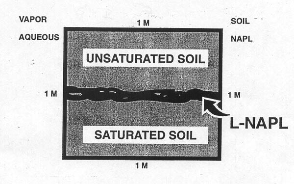
Introduction. The previous session provided a review of important multiphase flow concepts which govern the behavior of non aqueous phase liquids (NAPL’s) when they are released into the subsurface. Refer again to Figure I-1. Assume that the LNAPL or DNAPL has migrated through the subsurface and reached a more or less static configuration. Focus your attention on a small control volume, such as Figure I-10 below, which contains soil, water, NAPL and some air inside the free pore space.

 

Figure I-10.  This control volume is located at the surface of the water table in Figure I-1, on which a layer of LNAPL is floating. Initially organic compounds are assumed to be contained in the NAPL phase (i.e. initially when the NAPL is freshly spilled all the organic components are still in the NAPL). Over time individual organic compounds (contaminants) will partition out of the NAPL and migrate into the surrounding soil, water and air phases.

 

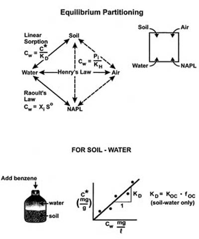
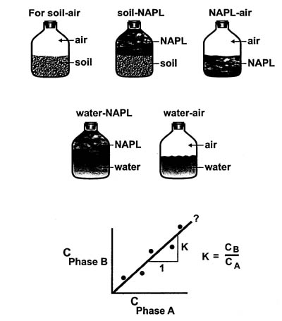
Figure I-10 provides the basis for developing a general approach to making equilibrium partitioning calculations. These calculations will tell us how a particular organic compound (initially entirely contained in the NAPL phase), will be distributed when chemical equilibrium has been reached. For example assume that the LNAPL in Figure I-10 is gasoline which is originally (before it is spilled) composed of 3% by weight of benzene ( a regulated contaminant). The equilibrium partitioning concepts and calculations which we are about to develop will provide estimates of how much benzene will be dissolved into the water phase, how much will be volatilized into air located in the free pore space, how much will be come sorbed to the soil phase, and finally how much benzene will remain in the NAPL phase, once chemical equilibrium has been reached. To further develop the partitioning concept consider the sealed laboratory flasks shown in Figure I-11 below.

 

Figure I-11.  Equilibrium Partitioning Pathways in a soil-air-water-NAPL system.  The sealed laboratory shake flasks experiments are designed to permit partitioning between two different phases.

 

If a known quantity of an organic compound, say benzene, is added for example to the flask containing soil and water, after equilibrium is reached some of the benzene will remain dissolved in the water phase and the rest will be adsorbed to the organic carbon in the soil phase. The benzene in the water phase could be measured in mg/l (C_w) and the benzene in the soil-sorbed phase could be quantified in mg/g, i.e. milligrams per gram of soil (C*), and plotted as shown in Figure I-11. The different points in Figure I-11 would come from adding different amounts of benzene to other soil-water flasks. If a straight line is fit through the origin, then the slope of the line, K, is equal to the ratio of C*/C_w.

Figure I-11 also indicates that similar experiments could be run by adding known amounts of benzene to the other five combinations of phases in the other flasks (i.e. air-soil, NAPL-soil, air-NAPL, etc). Linear "isotherm" plots would likewise yield "K" values which are simple ratios of the two phase concentrations in each experiment.

Figure I-11 illustrates how equilibrium partitioning ratios (K values), could be determined experimentally for each possible combination of soil, water, NAPL, and air phases using materials form a specific field site. Once known these K values could easily be used to answer the question of how a contaminant like benzene would partition under the conditions used in th e experimental analysis. However these experimental-derived partitioning coefficients obviously cannot used very well to extrapolate conditions at other field sites. Also, it should be fairly obvious that the experimentally-based process described in Figure I-11 will be extremely labor-intensive if repeated often. Therefore it is advantageous to consider the use of empirically derived partitioning relationships in the process at hand. There are three such empirical relationships:

· Linear sorption (soil-water partitioning)

· Henry’s Law (air-water partitioning)

· Raoult’s Law (water-NAPL partitioning)

· Mechanisms of sorption

· Sorption models and isotherms (Langmuir, Freundlich, and linear). Note that the linear sorption represents the simplest expression of equilibrium partitioning between soil and water.

· Retardation. This concept will be used later when we discuss contaminant plume migration. Don’t spend a lot of time on it now.

· Estimating the distribution coefficient K_D (page 143). This section provides further explanation of the concepts discussed above in Figure I-11. Note that K_D is modeled as the product of K_oc x f_oc. This is very important because it K_oc is a property (only) of the organic compound and f_oc is a property of the particular soil. Also not on page 146 that K_oc is related to K_om.

· Determine the coefficient of retardation using K_oc (page 146). Again we will use this concept later.

Henrys Law. Refer to section 3.6 in Wiedemeyer (page 153-154). Henry’s law basically states that the equilibrium concentration of the organic compound in air is directly proportional to the corresponding aqueous concentration. Henry’s law coefficient, H, (we used "K" in Figure I-11) is the proportionality constant with a unique value for a particular organic compound.

Raoult’s Law. Refer to pages 49-50 in Wiedemeyer. Note that Raoult’s Law was originally defined for mixtures of ideal gases. We are borrowing this concept here and using it to estimate the partitioning between NAPL and water. Wiedemeyer refers to Raoult’s Law in this case as the effective solubility relationship(page 49). It is clear that Raoult’s Law, as given by equation 2.11, is also a direct proportionality relationship. Here C_l is the same as C_w, or the concentration of organic compound in the aqueous phase.

In summary, this reading assignment has explained that the three equilibrium partitioning "laws" (Linear sorption, Henry’s Law and Raoult’s Law) are simple direct proportionality models which relate concentration in the soil, air, and NAPL phases to the corresponding concentration in the aqueous phase. We will now use these three laws to help us make quantitative estimates of equilibrium partitioning phenomena. Now refer to the partitioning pathway diagram shown at the top of Figure I-11.

The NAPL (gasoline for example, is a mixture of many individual organic compounds such a benzene, toluene ethylbenzene, etc. (unleaded gasoline may be composed of as many as 75 organic compounds). We now focus our attention on one compound of interest (benzene in the previous example) and ask the following question: If a known mass of benzene is initially added to the control volume in the NAPL phase what will be the mass of benzene in each of the four phases in the control volume after chemical equilibrium is reached? In other words how much benzene will partition out of the NAPL phase and ultimately appear in the soil, the water, and the air inside the pore space? The three solid lines in Figure I-11 show the pathways for which we have a partitioning law available. The dashed lines show partitioning pathways for which now law exits and, therefore these would have to be evaluated experimentally as is also shown in Figure I-11. Fortunately the three partitioning laws provide us with enough information to answer the above question with out resorting to significant experimentation.

The computational approach is illustrated in the Example problem given in Homework Problem I-11.  Go over this problem carefully taking care to understand how each solution step is accomplished.  Work problems I-11 and I-12 as instructed in the assignment sheet.

Equilibrium Partitioning Model (EPM):

Review the Equilibrium Partitioning Model Tutorial, then work problems I-13 and I-14 to complete the assignment on equilibrium partitioning.

Next Session | Previous Session | Table of Contents